sampleSizeCalc: A Comprehensive Guide to Sample Size Determination in Clinical Research

Introduction: The Lifeblood of Clinical Research

For clinical investigators, calculating sample size is often the most critical step when preparing grant proposals or IRB submissions.

Underpowered trials risk false-negative findings ($P > 0.05$), wasting research grants and patient effort. Conversely, overpowered trials waste resources and expose unnecessary subjects to experimental risks.

The sampleSizeCalc package supports the designs illustrated in 52 clinical scenarios below. Each example explains the population, study procedures, endpoint, planning assumptions, and how the result translates into recruitment.

These are teaching protocols. Except where a published numerical example is explicitly identified, clinical effects, standard deviations, event rates, and margins are illustrative assumptions. The methodological reference supports the formula; it does not establish those clinical inputs. A real protocol should document the source population, endpoint definition, follow-up window, and uncertainty of each planning input.

Numerical interpretations are evaluated from the R result objects when the site is built. Some diagnostic branches convert an unrounded requirement to a screening total; operational recruitment should also respect integer case and control quotas. Default reports contain the plain-text formula, LaTeX source, calculation process, and references.

Plain-English Glossary of Statistical Terms

$\alpha$ (Type I Error / False Positive): The probability of declaring a treatment effective when it truly is not — the “probability of convicting an innocent drug” (conventionally 0.05).
$\text{Power} = 1 - \beta$ (True Positive Detection): The probability of catching a true effect when it exists — the “probability of catching the real culprit” (routinely 0.80 or 0.90).
Continuous vs. Binary Endpoints: Continuous measures numerical values (systolic BP drop in mmHg, fasting glucose in mmol/L); binary measures event status (eradicated vs. not, cured vs. not).
Two-Sided vs. One-Sided: Two-sided tests for differences in either direction (classical RCTs); one-sided tests for non-inferiority and directional superiority.
Dropout Rate ($d$): Inflation formula $N_{\text{screen}} = \lceil N / (1 - d) \rceil$.

Unified Syntax: The Three-Axis Function `calculate()`

\[\texttt{calculate(design, task, outcome, ...)}\]

Axis 1 design: what type of study? ("rct", "paired", "cohort", "caseControl", "diagAccuracy", "diagAUC", "singleArmPhaseII", "bioequivalence", "clusterRCT", …)
Axis 2 task: what scientific question? ("test" hypothesis testing, "estimate" CI precision, "noninferiority", "superiority", "equivalence")
Axis 3 outcome: how is the endpoint measured? ("mean", "proportion", "survival", "auc", "rate", "ordinal", "lr", "correlation", "events")

Printing a result shows the formula in plain text and LaTeX, the calculation process, and references. summary() also lists all inputs, design axes, and recorded adjustments.

Chapter 1: Randomized Controlled Trials (RCTs)

1.1 Two Independent Means (Continuous Endpoint)

Population and decision: A cardiology service plans a blinded, parallel, 1:1 randomized trial in adults aged 40–75 whose background antihypertensive treatment is stable, comparing an add-on study drug with add-on placebo.
Procedures and endpoint: At baseline and week 12, use the same protocol to average repeated seated BP readings. The primary outcome is baseline minus week-12 systolic BP, so a larger positive change means greater improvement; each patient supplies one change score.
Planning inputs: Assume mean reductions of 10 and 12 mmHg and a common change-score SD of 3 mmHg. These map to mean1, mean2, and sd; the SD of baseline BP is not interchangeable with the SD of change. Verify these assumptions using comparable pilot or external data.
Why this design: The question is whether two independent mean changes differ, using two-sided α=0.05 and 80% power. The targeted between-group difference is 2 mmHg, distinct from either group’s reduction from baseline.
Formula: \[n = 2\left(\frac{(Z_{\alpha/2} + Z_{\beta}) \cdot \sigma}{\mu_1 - \mu_2}\right)^2\] Chow, Shao, Wang & Lokhnygina (2017), Sample Size Calculations in Clinical Research (3rd ed.), CRC Press.

res_1_1 <- calculate("rct", "test", "mean", mean1 = 10, mean2 = 12, sd = 3, alpha = 0.05, power = 0.8)
print(res_1_1)
#> ────────────────────────────────────────────────────────────────────────────────
#> ✔ Sample Size Calculation Results
#> • Design type: "Two independent samples, mean comparison"
#> • Sample size per group: 37
#> • Total sample size: 74
#> Formula (plain text):
#> `n = 2 * ((Z_alpha/2 + Z_beta) * sd / (mean1 - mean2))^2`
#> Formula (LaTeX):
#> $$n = 2\left(\frac{Z_{\alpha/2} + Z_{\beta}}{\delta}\right)^2 = 2\left(\frac{(Z_{\alpha/2} + Z_{\beta}) \cdot \sigma}{\mu_1 - \mu_2}\right)^2$$
#> Calculation process:
#> 
#> • Step 1: State hypotheses: H0: mu1 = mu2 vs H1: mu1 != mu2 (two-sided alpha =
#> 0.05, power = 0.80).
#> • Step 2: Calculate mean difference delta = |mu1 - mu2| = |10 - 12| = 2; common
#> SD sigma = 3.
#> • Step 3: Determine critical values: Z_(alpha/2) = 1.96 (for two-sided alpha =
#> 0.05), Z_beta = 0.8416 (for power = 0.80).
#> • Step 4: Compute initial sample size via normal approximation: n0 = 2 *
#> ((Z_(alpha/2) + Z_beta) * sigma / delta)^2 = 2 * ((1.96 + 0.8416) * 3 / 2)^2 =
#> 35.32.
#> • Step 5: Refine via exact two-sample Student's t-test power iteration
#> (accounting for degrees of freedom df = 2n - 2).
#> • Step 6: Round up to integer: n = 37 per group, total sample size N = 74.
#> Reference:
#> Chow, S. C., Shao, J., Wang, H., & Lokhnygina, Y. (2017). Sample Size Calculations in Clinical Research (3rd ed.). CRC Press. Chapter 3 (Comparing Means), Section 3.2.1 two-sample parallel design, Eq 3.11 (p. 48; the Student t refinement is Table 3.2, p. 49).
#> 
#>  Also: Machin et al. (2018) Eq 5.4, p. 69 (same formula with the Student t correction term).
#> ────────────────────────────────────────────────────────────────────────────────
#>

Result and recruitment: 37 analyzable patients per arm, 74 total. The report shows the normal approximation of about 35.32 per arm before the noncentral t calculation and rounding. If 10% are expected to lack the primary endpoint, plan 42 per arm (84 total); this additional adjustment is not included in the RCT result.

The four report components

Component	Console label	Result field
Plain-text formula	`Formula (plain text)`	`formula`
LaTeX source	`Formula (LaTeX)`	`formula_latex`
Calculation process	`Calculation process`	`calculation_steps` (alias `calculation`)
References	`Reference`	`reference`

res_1_1$formula
cat(res_1_1$formula_latex)
cat(res_1_1$calculation_steps, sep = "\n")
cat(res_1_1$reference)

The R console displays copyable LaTeX source. To typeset it in R Markdown, use cat(res_1_1$formula_latex) in a chunk with results = "asis". The reporting guide includes an executed example and instructions for saving the report.

1.2 Two Independent Proportions (Binary Endpoint)

Population and decision: A gastroenterology trial enrolls adults with confirmed H. pylori infection who are eligible for either of two 14-day regimens, with recent antibiotic use and previous eradication failure handled by prespecified eligibility rules.
Procedures and endpoint: Determine eradication with a standardized urea breath test in a fixed post-treatment window. Define medication restrictions, invalid tests, and repeat assessments in advance; improvement in symptoms at treatment completion is not the eradication endpoint.
Planning inputs: Illustrative rates are p1 = 0.85 and p2 = 0.70, an absolute difference of 15 percentage points. Actual sources must match treatment history, resistance setting, and the timing and definition of eradication.
Why this design: Different patients form the two groups, so use independent proportions with two-sided α=0.05 and 80% power. Prespecify how nonadherence and missing follow-up enter the analysis.
Formula (Fleiss asymptotic): \[n = \frac{\left[Z_{\alpha/2}\sqrt{2\bar{p}(1-\bar{p})} + Z_{\beta}\sqrt{p_1(1-p_1)+p_2(1-p_2)}\right]^2}{(p_1-p_2)^2}\] Fleiss, Tytun & Ury (1980), Biometrics 36(2), 343-346.

res_1_2 <- calculate("rct", "test", "proportion", p1 = 0.85, p2 = 0.70, alpha = 0.05, power = 0.8)
print(res_1_2)
#> ────────────────────────────────────────────────────────────────────────────────
#> ✔ Sample Size Calculation Results
#> • Design type: "Two independent proportions"
#> • Sample size per group: 121
#> • Total sample size: 242
#> Formula (plain text):
#> `n = (Z_a/2 * sqrt(2*p_bar*(1-p_bar)) + Z_b * sqrt(p1*(1-p1)+p2*(1-p2)))^2 /
#> (p1-p2)^2`
#> Formula (LaTeX):
#> $$n = \frac{\left[Z_{\alpha/2}\sqrt{2\bar{p}(1-\bar{p})} + Z_{\beta}\sqrt{p_1(1-p_1) + p_2(1-p_2)}\right]^2}{(p_1 - p_2)^2}$$
#> Calculation process:
#> 
#> • Step 1: State hypotheses: H0: p1 = p2 vs H1: p1 != p2 (two-sided alpha =
#> 0.05, power = 0.80).
#> • Step 2: Compute pooled proportion: p_bar = (p1 + p2) / 2 = (0.85 + 0.70) / 2
#> = 0.775.
#> • Step 3: Determine critical values: Z_(alpha/2) = 1.96, Z_beta = 0.8416.
#> • Step 4: Compute Fleiss formula numerator components:
#> Z_(alpha/2)*sqrt(2*p_bar*(1-p_bar)) = 1.1575; Z_beta*sqrt(p1(1-p1)+p2(1-p2)) =
#> 0.4889.
#> • Step 5: Calculate unrounded sample size per group: n = (1.1575 + 0.4889)^2 /
#> (0.85 - 0.70)^2 = 120.47.
#> • Step 6: Round up to integer: n = 121 per group, total sample size N = 242.
#> Reference:
#> Primary (formula as implemented, without continuity correction): Fleiss, J. L., Tytun, A., & Ury, H. K. (1980). A simple approximation for calculating sample sizes for comparing independent proportions. Biometrics, 36(2), 343-346.
#> 
#> With continuity correction: Casagrande, J. T., Pike, M. C., & Smith, P. G. (1978). An improved approximate formula for calculating sample sizes for comparing two binomial distributions. Biometrics, 34(3), 483-494.
#> 
#> Book: Fleiss, J. L., Levin, B., & Paik, M. C. (2003). Statistical methods for rates and proportions (3rd ed.). Wiley.
#> ────────────────────────────────────────────────────────────────────────────────
#>

Result and recruitment: 121 patients per arm, 242 total. Allowing for 10% missing primary endpoints gives 135 per arm and 270 total; the analysis population and missing-data strategy still require explicit definitions.

1.3 Survival Analysis (Log-Rank Test Events)

Population and decision: An oncology group plans a 1:1 randomized trial in advanced non-small-cell lung cancer patients eligible for both study regimens, with follow-up measured from randomization.
Procedures and endpoint: Specify overall survival as the primary outcome, with death from any cause as the event and last confirmed survival as the censoring date. Progression is not an overall-survival event; a progression-free survival design needs its own event definition and assumptions.
Planning inputs: Assume proportional hazards, hr = 0.70, experimental allocation pE = 0.50, two-sided α=0.05, and 80% power. A hazard ratio is not the ratio of two fixed-time death probabilities.
Why this design: First determine the number of deaths required. Accrual duration, additional follow-up, survival distributions, and losses then determine what fraction of recruited patients will contribute an event and when analysis is feasible.
Formula (Schoenfeld): \[E = \frac{(Z_{\alpha/2} + Z_{\beta})^2}{p_E(1 - p_E)[\ln(HR)]^2}\] Schoenfeld (1983), Biometrics 39(2), 499-503.

res_1_3 <- calculate("rct", "test", "survival", hr = 0.70, pE = 0.50, alpha = 0.05, power = 0.8)
print(res_1_3)
#> ────────────────────────────────────────────────────────────────────────────────
#> ✔ Sample Size Calculation Results
#> • Design type: "Survival (log-rank)"
#> • Events needed: 247
#> Formula (plain text):
#> `E = (Z_a/2 + Z_b)^2 / (pE*(1-pE)*log(HR)^2)`
#> Formula (LaTeX):
#> $$E = \frac{(Z_{\alpha/2} + Z_{\beta})^2}{p_E(1-p_E)[\ln(HR)]^2}$$
#> Calculation process:
#> 
#> • Step 1: State survival parameters: Hazard Ratio HR = 0.70, experimental arm
#> allocation pE = 0.50 (alpha = 0.05, power = 0.80).
#> • Step 2: Compute log hazard ratio: ln(HR) = ln(0.70) = -0.3567.
#> • Step 3: Determine critical values: Z_(alpha/2) = 1.96, Z_beta = 0.8416.
#> • Step 4: Apply Schoenfeld formula: E = (Z_(alpha/2) + Z_beta)^2 / [pE * (1 -
#> pE) * (ln HR)^2] = (1.96 + 0.8416)^2 / [0.50 * 0.50 * (-0.3567)^2] = 246.79.
#> • Step 5: Round up to integer: Target events needed E = 247.
#> Reference:
#> Primary: Schoenfeld, D. A. (1983). Sample-size formula for the proportional-hazards regression model. Biometrics, 39(2), 499-503.
#> 
#> Extensions:
#> - Hsieh, F. Y., & Lavori, P. W. (2000). Sample-size calculations for the Cox proportional hazards regression model with nonbinary covariates. Controlled Clinical Trials, 21(6), 552-560.
#> - Rubinstein, L. V., Gail, M. H., & Santner, T. J. (1981). Planning the duration of a comparative clinical trial with loss to follow-up and a period of continued observation. Journal of Chronic Diseases, 34(9-10), 469-479.
#> ────────────────────────────────────────────────────────────────────────────────
#>

Result and recruitment: 247 deaths are required. If a separate accrual and follow-up model predicts an event fraction of 60% at analysis, a rough resource estimate is 412 patients. That fraction is an additional assumption, not an output derived from HR by this function.

1.4 Non-Inferiority Trial (Continuous Mean)

Population and decision: A randomized parallel trial compares a lower-cost symptom-management strategy with usual care in patients with symptomatic diabetic peripheral neuropathy, while keeping background treatment stable.
Procedures and endpoint: Use improvement from baseline to week 12 on a prespecified symptom scale, with larger reductions indicating benefit. Standardize assessment and require sufficient baseline symptoms to avoid a pronounced floor effect.
Planning inputs: Assume improvements of 10 and 9.5 points, SD=3, and a maximum acceptable loss of margin = 1 point. Justify the margin using clinical importance and the established comparator effect; it should not be chosen from the anticipated difference alone.
Why this design: Demonstrate that study minus control improvement exceeds −1 point. This example uses one-sided α=0.05 and 80% power; a protocol choosing one-sided 0.025 must recalculate accordingly.
Formula: \[n = 2\left(\frac{(Z_{\alpha} + Z_{\beta})\sigma}{\mu_1 - \mu_2 + \Delta}\right)^2\] Chow et al. (2017), Chapter 4.

res_1_4 <- calculate("rct", "noninferiority", "mean", mean1 = 10, mean2 = 9.5, sd = 3, margin = 1, alpha = 0.05, power = 0.8)
print(res_1_4)
#> ────────────────────────────────────────────────────────────────────────────────
#> ✔ Sample Size Calculation Results
#> • Design type: "Non-inferiority (means)"
#> • Sample size per group: 50
#> • Total sample size: 100
#> Formula (plain text):
#> `n = 2*(Z_a+Z_b)^2*sd^2/(mean1-mean2+margin)^2`
#> Formula (LaTeX):
#> $$n = 2\left(\frac{(Z_{\alpha} + Z_{\beta})\sigma}{\mu_1 - \mu_2 + \Delta}\right)^2$$
#> Calculation process:
#> 
#> • Step 1: State non-inferiority hypotheses: H0: mu1 - mu2 <= -margin vs H1: mu1
#> - mu2 > -margin (margin Delta = 1, one-sided alpha = 0.05, power = 0.80).
#> • Step 2: Effective difference: delta_E = mu1 - mu2 + margin = 10 - 9.50 + 1 =
#> 1.50; SD sigma = 3.
#> • Step 3: Determine critical values: one-sided Z_alpha = 1.6449, Z_beta =
#> 0.8416.
#> • Step 4: Compute sample size: n = 2 * (Z_alpha + Z_beta)^2 * sigma^2 /
#> delta_E^2 = 2 * (1.6449 + 0.8416)^2 * 3^2 / (1.50)^2 = 49.46.
#> • Step 5: Round up to integer: n = 50 per group, total sample size N = 100.
#> Reference:
#> Chow, S. C., Shao, J., Wang, H., & Lokhnygina, Y. (2017). Sample Size Calculations in Clinical Research (3rd ed.). CRC Press. Chapter 3 (Comparing Means), Section 3.2.2 noninferiority, Eq 3.12, p. 50.
#> 
#>  Also: Machin et al. (2018) Eq 11.3, p. 173.
#> ────────────────────────────────────────────────────────────────────────────────
#>

Result and recruitment: 50 per arm, 100 total. Document the primary analysis population, adherence handling, and missing outcomes alongside the margin justification; they are part of the non-inferiority design.

1.5 Non-Inferiority Trial (Binary Endpoint)

Population and decision: An adult lower urinary tract infection trial compares a more convenient study regimen with an effective active comparator, using consistent microbiological and eligibility criteria.
Procedures and endpoint: Define clinical cure in a fixed post-treatment visit window, with prespecified rules for rescue treatment, antibiotic switching, and missing visits. Each patient contributes one binary outcome.
Planning inputs: Assume both cure rates are 85%, with a maximum acceptable absolute loss of 5 percentage points: p1 = p2 = 0.85, margin = 0.05. The margin is illustrative and requires clinical and effect-preservation justification.
Why this design: Use one-sided α=0.05 and 80% power to exclude an unacceptable reduction in cure. A nonsignificant ordinary difference test does not establish non-inferiority.
Formula: \[n = \frac{(Z_{\alpha}+Z_{\beta})^2\left[p_1(1-p_1)+p_2(1-p_2)\right]}{(p_1-p_2+\Delta)^2}\] Chow et al. (2017); Machin et al. (2018) Ch. 11.

res_1_5 <- calculate("rct", "noninferiority", "proportion", p1 = 0.85, p2 = 0.85, margin = 0.05, alpha = 0.05, power = 0.8)
print(res_1_5)
#> ────────────────────────────────────────────────────────────────────────────────
#> ✔ Sample Size Calculation Results
#> • Design type: "Non-inferiority (proportions)"
#> • Sample size per group: 631
#> • Total sample size: 1262
#> Parameter roles
#> 
#> • p1 = experimental-group response rate
#> • p2 = active-control response rate
#> • margin = non-inferiority margin Delta (one-sided alpha)
#> Formula (plain text):
#> `n = (Za+Zb)^2 * (p1q1+p2q2) / (p1-p2+margin)^2`
#> Formula (LaTeX):
#> $$n = \frac{(Z_{\alpha}+Z_{\beta})^2\left[p_1(1-p_1)+p_2(1-p_2)\right]}{(p_1-p_2+\Delta)^2}$$
#> Calculation process:
#> 
#> • Step 1: State non-inferiority hypotheses: H0: p1 - p2 <= -margin vs H1: p1 -
#> p2 > -margin (margin Delta = 0.05, one-sided alpha = 0.05, power = 0.80).
#> • Step 2: Effective difference: delta_E = p1 - p2 + margin = 0.85 - 0.85 + 0.05
#> = 0.05.
#> • Step 3: Determine critical values: one-sided Z_alpha = 1.6449, Z_beta =
#> 0.8416.
#> • Step 4: Compute sample size: n = (Z_alpha + Z_beta)^2 * [p1(1-p1) + p2(1-p2)]
#> / delta_E^2 = 630.62.
#> • Step 5: Round up to integer: n = 631 per group, total sample size N = 1262.
#> Reference:
#> Primary: Chow, S. C., Shao, J., Wang, H., & Lokhnygina, Y. (2017). Sample Size Calculations in Clinical Research (3rd ed.). CRC Press. Chapter 4 (Large Sample Tests for Proportions), Section 4.2.2 noninferiority/superiority, Eq 4.8 (p. 78).
#> 
#>  Also: Machin et al. (2018) Chapter 11, Eq 11.5-11.6, p. 174.
#> ────────────────────────────────────────────────────────────────────────────────
#>

Result and recruitment: 631 per arm, 1262 total. If endpoint completeness is expected to be 90%, plan 702 per arm. Treatment failures should not be removed from the denominator as though they were recruitment losses.

1.6 Superiority Trial (Continuous Mean)

Population and decision: A knee osteoarthritis trial randomizes patients with sufficient baseline pain to a study topical preparation or active comparator, seeking improvement beyond a prespecified clinically relevant difference.
Procedures and endpoint: Measure baseline-to-week-12 reduction on a specified WOMAC pain subscale, with standardized assessments and rules for rescue medication before measurement.
Planning inputs: Assume reductions of 12 versus 10 points, SD=3, and margin = 1 point. The effective difference is 12−10−1=1 point; using the full anticipated 2-point difference in the denominator would answer a different question.
Why this design: This is superiority beyond a positive margin, with one-sided α=0.05 and 80% power. Specify the scale version, score direction, and clinical reasoning for the margin before observing results.
Formula: \[n = 2\left(\frac{(Z_{\alpha} + Z_{\beta})\sigma}{\mu_1 - \mu_2 - \Delta}\right)^2\] Chow et al. (2017).

res_1_6 <- calculate("rct", "superiority", "mean", mean1 = 12, mean2 = 10, sd = 3, margin = 1, alpha = 0.05, power = 0.8)
print(res_1_6)
#> ────────────────────────────────────────────────────────────────────────────────
#> ✔ Sample Size Calculation Results
#> • Design type: "Superiority (means)"
#> • Sample size per group: 112
#> • Total sample size: 224
#> Formula (plain text):
#> `n = 2*(Z_a+Z_b)^2*sd^2/(mean1-mean2-margin)^2`
#> Formula (LaTeX):
#> $$n = 2\left(\frac{(Z_{\alpha} + Z_{\beta})\sigma}{\mu_1 - \mu_2 - \Delta}\right)^2$$
#> Calculation process:
#> 
#> • Step 1: State superiority hypotheses: H0: mu1 - mu2 <= margin vs H1: mu1 -
#> mu2 > margin (margin Delta = 1, one-sided alpha = 0.05, power = 0.80).
#> • Step 2: Effective difference: delta_E = mu1 - mu2 - margin = 12 - 10 - 1 = 1;
#> SD sigma = 3.
#> • Step 3: Determine critical values: one-sided Z_alpha = 1.6449, Z_beta =
#> 0.8416.
#> • Step 4: Compute sample size: n = 2 * (Z_alpha + Z_beta)^2 * sigma^2 /
#> delta_E^2 = 2 * (1.6449 + 0.8416)^2 * 3^2 / (1)^2 = 111.29.
#> • Step 5: Round up to integer: n = 112 per group, total sample size N = 224.
#> Reference:
#> Chow, S. C., Shao, J., Wang, H., & Lokhnygina, Y. (2017). Sample Size Calculations in Clinical Research (3rd ed.). CRC Press. Chapter 3 (Comparing Means), Section 3.2.2 superiority, Eq 3.12, p. 50.
#> 
#>  Also: Machin et al. (2018) Eq 11.3, p. 173.
#> ────────────────────────────────────────────────────────────────────────────────
#>

Result and recruitment: 112 per arm, 224 total. Recruitment must deliver the required primary endpoints; changing the margin after observing outcomes would change the original scientific question.

1.7 Superiority Trial (Binary Endpoint)

Population and decision: A dermatology trial compares two oral regimens in patients with confirmed toenail onychomycosis, defining one target nail per patient for the primary analysis.
Procedures and endpoint: Evaluate complete cure at a fixed long-term visit, such as week 52, requiring both clinical clearing and mycological negativity. End-of-treatment cosmetic improvement is not the same endpoint.
Planning inputs: Assume cure rates of 30% and 20%, and require the difference to exceed 5 percentage points: p1 = 0.30, p2 = 0.20, margin = 0.05. The remaining effective difference is 0.05.
Why this design: Use one-sided α=0.05 and 80% power for superiority beyond the margin. Parameter sources should match severity, previous treatment, cure definition, and follow-up duration.
Formula: \[n = \frac{(Z_{\alpha}+Z_{\beta})^2\left[p_1(1-p_1)+p_2(1-p_2)\right]}{(p_1-p_2-\Delta)^2}\] Chow et al. (2017).

res_1_7 <- calculate("rct", "superiority", "proportion", p1 = 0.30, p2 = 0.20, margin = 0.05, alpha = 0.05, power = 0.8)
print(res_1_7)
#> ────────────────────────────────────────────────────────────────────────────────
#> ✔ Sample Size Calculation Results
#> • Design type: "Superiority (proportions)"
#> • Sample size per group: 916
#> • Total sample size: 1832
#> Formula (plain text):
#> `n = (Z_alpha + Z_beta)^2 * (p1*(1-p1) + p2*(1-p2)) / (p1 - p2 - margin)^2`
#> Formula (LaTeX):
#> $$n = \frac{(Z_{\alpha} + Z_{\beta})^2[p_1(1-p_1) + p_2(1-p_2)]}{(p_1 - p_2 - \Delta)^2}$$
#> Calculation process:
#> 
#> • Step 1: State superiority hypotheses: H0: p1 - p2 <= margin vs H1: p1 - p2 >
#> margin (margin Delta = 0.05, one-sided alpha = 0.05, power = 0.80).
#> • Step 2: Effective difference: delta_E = p1 - p2 - margin = 0.30 - 0.20 - 0.05
#> = 0.05.
#> • Step 3: Determine critical values: one-sided Z_alpha = 1.6449, Z_beta =
#> 0.8416.
#> • Step 4: Compute sample size: n = (Z_alpha + Z_beta)^2 * [p1(1-p1) + p2(1-p2)]
#> / delta_E^2 = (1.6449 + 0.8416)^2 * [0.21 + 0.16] / (0.05)^2 = 915.02.
#> • Step 5: Round up to integer: n = 916 per group, total sample size N = 1832.
#> Reference:
#> Chow, S. C., Shao, J., Wang, H., & Lokhnygina, Y. (2017). Sample Size Calculations in Clinical Research (3rd ed.). CRC Press. Chapter 4 (Large Sample Tests for Proportions), Section 4.2.2 noninferiority/ superiority, Eq 4.8 (p. 78).
#> 
#>  Also: Machin et al. (2018) Eq 11.5-11.6, p. 174; Fleiss, Tytun & Ury (1980), Biometrics 36(2), 343-346.
#> ────────────────────────────────────────────────────────────────────────────────
#>

Result and recruitment: 916 per arm, 1832 total. If 10% lack the long-term endpoint, plan 1018 per arm and ensure sufficient follow-up visit capacity.

1.8 Equivalence Trial (Continuous Mean)

Population and decision: A parallel randomized study compares two formulations in patients with stable hypothyroidism and stable background dosing, allowing sufficient time for the prespecified steady-state assessment.
Procedures and endpoint: This teaching example uses mean steady-state total serum thyroxine, with standardized sampling time and laboratory platform. It illustrates equivalence of a continuous pharmacodynamic endpoint, not a complete bioequivalence or interchangeability assessment.
Planning inputs: Assume means of 10 and 10.2 μg/dL, SD=3 μg/dL, and an equivalence corridor of ±1 μg/dL. The SD and margins require endpoint-specific clinical and pilot evidence.
Why this design: Both unacceptable directions must be excluded using equivalence testing, with one-sided α=0.05 and target power 80%. Failure to find a difference does not establish equivalence.
Formula (TOST): \[n = 2\left(\frac{(Z_{\alpha} + Z_{\beta/2})\sigma}{\Delta - |\mu_1 - \mu_2|}\right)^2\] Chow et al. (2017).

res_1_8 <- calculate("rct", "equivalence", "mean", mean1 = 10, mean2 = 10.2, sd = 3, margin = 1, alpha = 0.05, power = 0.8)
print(res_1_8)
#> ────────────────────────────────────────────────────────────────────────────────
#> ✔ Sample Size Calculation Results
#> • Design type: "Equivalence (means)"
#> • Sample size per group: 241
#> • Total sample size: 482
#> Formula (plain text):
#> `n = 2*(Z_a+Z_b/2)^2*sd^2/(margin-|mean1-mean2|)^2`
#> Formula (LaTeX):
#> $$n = 2\left(\frac{(Z_{\alpha} + Z_{\beta/2})\sigma}{\Delta - |\mu_1 - \mu_2|}\right)^2$$
#> Calculation process:
#> 
#> • Step 1: State equivalence hypotheses (TOST): H0: |mu1 - mu2| >= margin vs H1:
#> |mu1 - mu2| < margin (margin Delta = 1, alpha = 0.05, power = 0.80).
#> • Step 2: Margin clearance: Delta - |mu1 - mu2| = 1 - |10 - 10.20| = 0.80; SD
#> sigma = 3.
#> • Step 3: Determine critical values: one-sided Z_alpha = 1.6449, Z_(beta/2) =
#> 1.2816.
#> • Step 4: Compute sample size: n = 2 * (Z_alpha + Z_(beta/2))^2 * sigma^2 /
#> (Delta - |mu1 - mu2|)^2 = 2 * (1.6449 + 1.2816)^2 * 3^2 / (0.80)^2 = 240.86.
#> • Step 5: Round up to integer: n = 241 per group, total sample size N = 482.
#> Reference:
#> Chow, S. C., Shao, J., Wang, H., & Lokhnygina, Y. (2017). Sample Size Calculations in Clinical Research (3rd ed.). CRC Press. Chapter 3 (Comparing Means), Section 3.2.3 equivalence, Eq 3.13, p. 51; the Z_{beta/2} convention is discussed in Section 3.6.1 (p. 67).
#> 
#>  Also: Machin et al. (2018) Eq 11.5-11.6, p. 174.
#> ────────────────────────────────────────────────────────────────────────────────
#>

Result and recruitment: 241 per arm, 482 total. This requirement concerns the single defined continuous endpoint; additional primary or pharmacokinetic outcomes need their own planning.

1.9 Equivalence Trial (Binary Endpoint)

Population and decision: An anesthesia service randomizes adults undergoing the same type of surgery to two postoperative analgesic regimens, asking whether a more convenient regimen provides sufficiently similar response rates.
Procedures and endpoint: Define success in advance, for example meeting a specified pain-reduction threshold without rescue medication during the first 6 hours. Prespecify rescue use, early withdrawal, and how repeated pain observations form one patient-level result.
Planning inputs: Assume response rates of 50% and 52%, with an equivalence corridor of ±10 percentage points: p1 = 0.50, p2 = 0.52, margin = 0.10.
Why this design: Use equivalence of independent proportions, one-sided α=0.05 and 80% power. The margin must be justified for this response definition rather than treated as a universal analgesic standard.
Formula: \[n = \frac{(Z_{\alpha}+Z_{\beta/2})^2\left[p_1(1-p_1)+p_2(1-p_2)\right]}{(\Delta-|p_1-p_2|)^2}\] Chow et al. (2017).

res_1_9 <- calculate("rct", "equivalence", "proportion", p1 = 0.50, p2 = 0.52, margin = 0.10, alpha = 0.05, power = 0.8)
print(res_1_9)
#> ────────────────────────────────────────────────────────────────────────────────
#> ✔ Sample Size Calculation Results
#> • Design type: "Equivalence (proportions)"
#> • Sample size per group: 669
#> • Total sample size: 1338
#> Formula (plain text):
#> `n = (Z_alpha + Z_beta/2)^2 * (p1*(1-p1) + p2*(1-p2)) / (margin - |p1 - p2|)^2`
#> Formula (LaTeX):
#> $$n = \frac{(Z_{\alpha} + Z_{\beta/2})^2[p_1(1-p_1) + p_2(1-p_2)]}{(\Delta - |p_1-p_2|)^2}$$
#> Calculation process:
#> 
#> • Step 1: State equivalence hypotheses (TOST): H0: |p1 - p2| >= margin vs H1:
#> |p1 - p2| < margin (margin Delta = 0.10, alpha = 0.05, power = 0.80).
#> • Step 2: Margin clearance: Delta - |p1 - p2| = 0.10 - |0.50 - 0.52| = 0.08.
#> • Step 3: Determine critical values: one-sided Z_alpha = 1.6449, Z_(beta/2) =
#> 1.2816.
#> • Step 4: Compute sample size: n = (Z_alpha + Z_(beta/2))^2 * [p1(1-p1) +
#> p2(1-p2)] / (Delta - |p1 - p2|)^2 = 668.52.
#> • Step 5: Round up to integer: n = 669 per group, total sample size N = 1338.
#> Reference:
#> Chow, S. C., Shao, J., Wang, H., & Lokhnygina, Y. (2017). Sample Size Calculations in Clinical Research (3rd ed.). CRC Press. Chapter 4 (Large Sample Tests for Proportions), Section 4.2.3 equivalence, Eq 4.9 (p. 79).
#> 
#>  Also: Machin et al. (2018) Eq 11.5-11.6, p. 174.
#> ────────────────────────────────────────────────────────────────────────────────
#>

Result and recruitment: 669 per arm, 1338 total. The count is independent patients with primary outcomes, not the number of repeated pain assessments.

Chapter 2: Paired, Single-Arm, and Crossover Trials

2.1 Paired Means (Pre- vs. Post-Treatment)

Population and decision: A rehabilitation clinic follows the same chronic low-back pain patients before and after a 6-week standardized exercise program, using a 0–10 pain scale.
Procedures and endpoint: Define improvement as baseline minus week-6 score and use consistent measurement conditions. Each patient’s two scores must be linkable to form one paired difference.
Planning inputs: Assume mean improvement meanDiff = 2 points and difference-score SD sdDiff = 3. Estimate the latter from paired pilot data; neither the baseline nor follow-up SD alone is an appropriate substitute.
Why this design: Use a two-sided paired-mean calculation with α=0.05 and 80% power. A before–after study estimates change; separating treatment effects from natural history requires an appropriate comparator design.
Formula: \[n = \left(\frac{(Z_{\alpha/2} + Z_{\beta}) \cdot \sigma_d}{\mu_d}\right)^2\] Rosner (2015), Fundamentals of Biostatistics (8th ed.).

res_2_1 <- calculate("paired", "test", "mean", meanDiff = 2, sdDiff = 3, alpha = 0.05, power = 0.8)
print(res_2_1)
#> ────────────────────────────────────────────────────────────────────────────────
#> ✔ Sample Size Calculation Results
#> • Design type: "Paired means"
#> • Pairs needed: 20
#> • Total individuals: 40
#> Formula (plain text):
#> `n = ((Z_a/2 + Z_b) * sd_diff / mean_diff)^2`
#> Formula (LaTeX):
#> $$n = \left(\frac{(Z_{\alpha/2} + Z_{\beta}) \cdot \sigma_d}{\mu_d}\right)^2$$
#> Calculation process:
#> 
#> • Step 1: State paired difference hypotheses: H0: mu_d = 0 vs H1: mu_d != 0
#> (alpha = 0.05, power = 0.80).
#> • Step 2: Expected paired difference mu_d = 2, SD of differences sigma_d = 3.
#> • Step 3: Determine critical values: Z_(alpha/2) = 1.96, Z_beta = 0.8416.
#> • Step 4: Normal approximation: n0 = ((Z_(alpha/2) + Z_beta) * sigma_d /
#> mu_d)^2 = ((1.96 + 0.8416) * 3 / 2)^2 = 17.66.
#> • Step 5: Exact paired Student's t-test degrees of freedom iteration.
#> • Step 6: Round up to integer: n = 20 pairs (total individuals = 40).
#> Reference:
#> Rosner, B. (2015). *Fundamentals of biostatistics* (8th ed.). Cengage Learning.
#> ────────────────────────────────────────────────────────────────────────────────
#>

Result and recruitment: 20 patients must complete both assessments, giving 40 measurements. A pair means two observations from one patient here. With 90% paired completion, recruit 23 patients.

2.2 Paired Binary Outcomes (McNemar / Connor)

Population and decision: A chronic-disease clinic introduces a medication reminder program in one cohort and compares adherence success before the program and at week 8.
Procedures and endpoint: Apply the same prespecified adherence threshold in both periods. Each patient forms a paired binary record; the question is whether success rises from 60% to 80%, not a comparison of independent cohorts.
Planning inputs: Set post-program p1 = 0.80, baseline p2 = 0.60, and discordant proportion psi = 0.25. This implies about 22.5% changing from failure to success and 2.5% changing in the opposite direction; verify that pattern using paired pilot records.
Why this design: McNemar/Connor planning uses the discordant pairs, with two-sided α=0.05 and 80% power. Both measurements are needed for a complete pair.
Formula (Connor): \[n = \frac{\left[Z_{\alpha/2}\sqrt{\psi} + Z_{\beta}\sqrt{\psi-\delta^2}\right]^2}{\delta^2}, \quad \delta = |p_1-p_2|\] Connor (1987), Biometrics 43(1), 207-211.

res_2_2 <- calculate("paired", "test", "proportion", p1 = 0.80, p2 = 0.60, psi = 0.25, alpha = 0.05, power = 0.8)
print(res_2_2)
#> ────────────────────────────────────────────────────────────────────────────────
#> ✔ Sample Size Calculation Results
#> • Design type: "Paired binary outcomes (McNemar / Connor)"
#> • Total sample size: 94
#> • Pairs needed: 47
#> Parameter roles
#> 
#> • p1/p2 = expected proportions (or sensitivities) in pairs
#> • psi = expected discordant-pair proportion (pi10 + pi01)
#> • output is in PAIRS (n individuals = 2 x pairs)
#> Formula (plain text):
#> `n = [Za*sqrt(psi) + Zb*sqrt(psi-delta^2)]^2/delta^2`
#> Formula (LaTeX):
#> $$n = \frac{\left[Z_{\alpha/2}\sqrt{\psi} + Z_{\beta}\sqrt{\psi-\delta^2}\right]^2}{\delta^2}$$
#> Calculation process:
#> 
#> • Step 1: Paired binary parameters: p1 = 0.80, p2 = 0.60, discordant pair
#> proportion psi = 0.25, difference delta = |p1 - p2| = 0.20.
#> • Step 2: Determine critical values: Z_(alpha/2) = 1.96, Z_beta = 0.8416.
#> • Step 3: Connor formula: n_pairs = [Z_(alpha/2)*sqrt(psi) + Z_beta*sqrt(psi -
#> delta^2)]^2 / delta^2 = 46.63.
#> • Step 4: Round up to integer: Pairs needed = 47.
#> Reference:
#> Primary: Connor, R. J. (1987). Sample size for testing differences in proportions for the paired-sample design. Biometrics, 43(1), 207-211.
#> 
#>  Also: Akoglu, H. (2022). Turkish Journal of Emergency Medicine, 22(4), Table 2 Eq 3b + Tables 6A/6B (uncorrected and Yates-corrected values).
#> ────────────────────────────────────────────────────────────────────────────────
#>

Result and recruitment: 47 patients with complete pairs, or 94 assessments. At 90% paired completion, recruit 53 patients; doubling the observations does not double the number of distinct people.

2.3 Single-Arm Mean vs. Historical Benchmark

Population and decision: A rare-disease rehabilitation project evaluates exercise endurance after a training program, using a comparable historical mean as a fixed benchmark because recruitment is limited.
Procedures and endpoint: Measure fully observed endurance duration in a standardized constant-load exercise test at week 8, in minutes. This is a continuous functional endpoint, not a censored survival time; historical and new cohorts need comparable severity, workloads, and stopping rules.
Planning inputs: Treat the historical mean as mu0 = 10 minutes, anticipate mu1 = 12, and assume sigma = 3, with two-sided α=0.05 and 80% power.
Why this design: This approximation treats the reference mean as known without error. A small or poorly matched historical sample requires a design that incorporates its uncertainty rather than treating a survival median as a known mean.
Formula: \[n = \frac{(Z_{\alpha/2} + Z_{\beta})^2 \sigma^2}{(\mu_1 - \mu_0)^2}\] Machin et al. (2018), Chapter 5.

res_2_3 <- calculate("rctSingleArm", "test", "mean", mu0 = 10, mu1 = 12, sigma = 3, alpha = 0.05, power = 0.8)
print(res_2_3)
#> ────────────────────────────────────────────────────────────────────────────────
#> ✔ Sample Size Calculation Results
#> • Design type: "Single-arm trial (continuous, vs fixed value)"
#> • Required sample size: 18
#> Parameter roles
#> 
#> • mu0 = reference/historical control mean (the null value)
#> • mu1 = anticipated treatment mean
#> • sigma = population standard deviation
#> Formula (plain text):
#> `n = (Za/2 + Zb)^2 * sigma^2 / (mu1-mu0)^2`
#> Formula (LaTeX):
#> $$n = \frac{(Z_{\alpha/2} + Z_{\beta})^2 \sigma^2}{(\mu_1 - \mu_0)^2}$$
#> Calculation process:
#> 
#> • Step 1: Single-arm continuous hypotheses: H0: mu = 10 vs H1: mu = 12, SD
#> sigma = 3 (alpha = 0.05, power = 0.80).
#> • Step 2: Effect size delta = |mu1 - mu0| = |12 - 10| = 2.
#> • Step 3: Determine critical values: Z_(alpha/2) = 1.96, Z_beta = 0.8416.
#> • Step 4: Sample size: n = (Z_(alpha/2) + Z_beta)^2 * sigma^2 / delta^2 = (1.96
#> + 0.8416)^2 * 3^2 / (2)^2 = 17.66.
#> • Step 5: Round up to integer: Required sample size n = 18.
#> Reference:
#> Primary: Machin, D., Campbell, M. J., Tan, S. B., & Tan, S. H. (2018). Sample Sizes for Clinical, Laboratory and Epidemiology Studies (4th ed.). Wiley. Chapter 5 (Continuous Outcomes, single-sample comparison).
#> ────────────────────────────────────────────────────────────────────────────────
#>

Result and recruitment: 18 patients with the defined endpoint. If 10% cannot complete the exercise assessment, plan 20 recruits; comparability of the reference remains central to interpretation.

2.4 Single-Arm Proportion vs. Historical Benchmark

Population and decision: An exploratory single-arm study enrolls relapsed/refractory lymphoma patients with defined prior treatment lines, comparing a new protocol with a fixed historical response rate.
Procedures and endpoint: Assess objective response at day 90 using consistent criteria. Prespecify deaths before assessment, rescue treatment, and unevaluable patients; restricting the denominator to surviving imaged patients changes the endpoint.
Planning inputs: Use teaching assumptions p0 = 0.70 and p1 = 0.80. Actual evidence must match treatment line, response definition, and assessment window to avoid an inappropriate historical comparator.
Why this design: This example uses a two-sided normal approximation with α=0.05 and 80% power. For an exact one-sided success cutoff or interim futility decision, consider the following A’Hern or Simon examples.
Formula: \[n = \frac{\left[Z_{\alpha/2}\sqrt{p_0(1-p_0)} + Z_{\beta}\sqrt{p_1(1-p_1)}\right]^2}{(p_1-p_0)^2}\] Hajian-Tilaki (2014), Eq 6.8.

res_2_4 <- calculate("rctSingleArm", "test", "proportion", p0 = 0.70, p1 = 0.80, alpha = 0.05, power = 0.8)
print(res_2_4)
#> ────────────────────────────────────────────────────────────────────────────────
#> ✔ Sample Size Calculation Results
#> • Design type: "Single-arm trial (binary, vs fixed value)"
#> • Required sample size: 153
#> Parameter roles
#> 
#> • p0 = null/historical control proportion
#> • p1 = anticipated treatment proportion
#> Formula (plain text):
#> `n = [Za*sqrt(p0q0) + Zb*sqrt(p1q1)]^2/(p1-p0)^2`
#> Formula (LaTeX):
#> $$n = \frac{\left[Z_{\alpha/2}\sqrt{p_0(1-p_0)} + Z_{\beta}\sqrt{p_1(1-p_1)}\right]^2}{(p_1 - p_0)^2}$$
#> Calculation process:
#> 
#> • Step 1: Single-arm binary hypotheses: H0: p = 0.70 vs H1: p = 0.80 (alpha =
#> 0.05, power = 0.80).
#> • Step 2: Determine critical values: Z_(alpha/2) = 1.96, Z_beta = 0.8416.
#> • Step 3: Sample size: n = [Z_(alpha/2)*sqrt(p0*q0) + Z_beta*sqrt(p1*q1)]^2 /
#> (p1 - p0)^2 = 152.48.
#> • Step 4: Round up to integer: Required sample size n = 153.
#> Reference:
#> Primary: Hajian-Tilaki, K. (2014). Sample size estimation in diagnostic test studies of biomedical informatics. Journal of Biomedical Informatics, 48, 193-204 (Eq 6.8; worked example 0.70 vs 0.80 -> n=153).
#> 
#>  Also: Akoglu, H. (2022). Table 2, Equation 2; Machin et al. (2018) Ch.3.
#> ────────────────────────────────────────────────────────────────────────────────
#>

Result and recruitment: 153 patients with ascertainable primary outcomes. This count addresses the planned distinction between 70% and 80%; it does not promise that the eventual response rate will equal the alternative.

2.5 Phase II Simon’s Optimal Two-Stage Design

Population and decision: A single-arm phase-II sarcoma study enrolls patients with measurable advanced disease and consistent previous treatment eligibility, seeking early termination when the regimen has inadequate activity.
Procedures and endpoint: Confirm objective response at approximately 8 weeks using prespecified criteria. Allow stage-1 patients to reach the assessment window and verify their outcomes before the formal continuation decision.
Planning inputs: Set an unacceptable response rate p0 = 0.10, a promising rate p1 = 0.30, one-sided α=0.05, and 80% power. Both rates must refer to the same disease subgroup and response definition.
Why this design: optimizer = "optimal" minimizes expected enrollment under the null, potentially accepting a larger maximum total than the minimax design.
Formula: exact binomial enumeration (Simon 1989). The design $(r_1/n_1, r/n)$ satisfies \[P_p(\text{reject }H_0) = \sum_{x_1=r_1+1}^{n_1}\binom{n_1}{x_1}p^{x_1}(1-p)^{n_1-x_1}\,P_p(X_2 > r-x_1), \quad P_{p_0}(\text{reject }H_0)\le\alpha\] and the analogous expression under $p_1$ must reach the target power. Simon (1989), Controlled Clinical Trials 10(1), 1-10.

res_2_5 <- calculate("singleArmPhaseII", "test", "proportion", p0 = 0.10, p1 = 0.30, alpha = 0.05, power = 0.8, optimizer = "optimal")
print(res_2_5)
#> ────────────────────────────────────────────────────────────────────────────────
#> ✔ Sample Size Calculation Results
#> • Design type: "Single-arm phase II (Simon two-stage, optimal)"
#> • Stage 1 sample size: 10
#> • Stage 1 futility boundary (stop if responses <= r1): 1
#> • Total sample size (both stages): 29
#> • Overall boundary (declare effective if responses > r): 5
#> Parameter roles
#> 
#> • p0 = unacceptable response rate (null)
#> • p1 = desirable response rate (alternative)
#> • stage 1: stop for futility if responses <= r_stage_1 of n_stage_1
#> • overall: declare effective if responses > r_total of n_total
#> Formula (plain text):
#> `exact binomial: P(effective|p0) <= alpha and P(effective|p1) >= power`
#> Formula (LaTeX):
#> $$P(\text{reject } H_0 \mid p_0) \le \alpha \quad \text{and} \quad P(\text{reject } H_0 \mid p_1) \ge 1-\beta$$
#> Calculation process:
#> 
#> • Step 1: State phase II hypotheses: H0: p <= 0.10 (unacceptable) vs H1: p >=
#> 0.30 (promising) (alpha = 0.05, power = 0.80).
#> • Step 2: Exhaustive exact binomial search under 'optimal' criterion.
#> • Step 3: Stage 1: Accrue n1 = 10 patients; stop early for futility if
#> responses <= r1 = 1.
#> • Step 4: Stage 2: If > 1 responses observed, accrue additional 19 patients up
#> to total n = 29.
#> • Step 5: Final decision: Declare effective if total responses > r = 5
#> (Expected sample size under H0 = 15).
#> Reference:
#> Primary: Simon, R. (1989). Optimal two-stage designs for phase II clinical trials. Controlled Clinical Trials, 10(1), 1-10.
#> 
#>  Also: Machin et al. (2018) Chapter 17 (Therapeutic Exploratory Trials).
#> ────────────────────────────────────────────────────────────────────────────────
#>

Result and stopping rules: Enroll 10 initially and stop for futility if responses are ≤1. Otherwise add 19 patients to a maximum of 29. Reject the null only if total responses exceed 5 (at least 6). Stage 1 is included in the maximum total.

2.6 Phase II Simon’s Minimax Two-Stage Design

Population and decision: A center addresses the same advanced sarcoma response question but has a firm ceiling on drug supply and eligible patients, making the worst-case enrollment especially important.
Procedures and endpoint: Use the same response definition and assessment window, with a prespecified stage-wise continuation rule. Do not switch optimization criteria after examining interim responses.
Planning inputs: Keep p0 = 0.10, p1 = 0.30, α=0.05, and 80% power, changing only optimizer = "minimax" so resource comparisons use the same error constraints.
Why this design: Minimax minimizes the maximum total sample size, not necessarily the expected number under the null. Compare both criteria when budgeting assessments and medication.

res_2_6 <- calculate("singleArmPhaseII", "test", "proportion", p0 = 0.10, p1 = 0.30, alpha = 0.05, power = 0.8, optimizer = "minimax")
print(res_2_6)
#> ────────────────────────────────────────────────────────────────────────────────
#> ✔ Sample Size Calculation Results
#> • Design type: "Single-arm phase II (Simon two-stage, minimax)"
#> • Stage 1 sample size: 15
#> • Stage 1 futility boundary (stop if responses <= r1): 1
#> • Total sample size (both stages): 25
#> • Overall boundary (declare effective if responses > r): 5
#> Parameter roles
#> 
#> • p0 = unacceptable response rate (null)
#> • p1 = desirable response rate (alternative)
#> • stage 1: stop for futility if responses <= r_stage_1 of n_stage_1
#> • overall: declare effective if responses > r_total of n_total
#> ! Multiple designs may achieve the minimum total sample size N;
#> ! this implementation selects the design minimizing Type I error (alpha) among ties.
#> 
#> Formula (plain text):
#> `exact binomial: P(effective|p0) <= alpha and P(effective|p1) >= power`
#> Formula (LaTeX):
#> $$P(\text{reject } H_0 \mid p_0) \le \alpha \quad \text{and} \quad P(\text{reject } H_0 \mid p_1) \ge 1-\beta$$
#> Calculation process:
#> 
#> • Step 1: State phase II hypotheses: H0: p <= 0.10 (unacceptable) vs H1: p >=
#> 0.30 (promising) (alpha = 0.05, power = 0.80).
#> • Step 2: Exhaustive exact binomial search under 'minimax' criterion.
#> • Step 3: Stage 1: Accrue n1 = 15 patients; stop early for futility if
#> responses <= r1 = 1.
#> • Step 4: Stage 2: If > 1 responses observed, accrue additional 10 patients up
#> to total n = 25.
#> • Step 5: Final decision: Declare effective if total responses > r = 5
#> (Expected sample size under H0 = 19.50).
#> Reference:
#> Primary: Simon, R. (1989). Optimal two-stage designs for phase II clinical trials. Controlled Clinical Trials, 10(1), 1-10.
#> 
#>  Also: Machin et al. (2018) Chapter 17 (Therapeutic Exploratory Trials).
#> ────────────────────────────────────────────────────────────────────────────────
#>

Result and stopping rules: Stage 1 enrolls 15, stopping if responses are ≤1; the maximum total is 25, with rejection requiring more than 5 responses. Compare that maximum with the optimal design’s 29 patients.

2.7 A’Hern Exact Single-Stage Binomial Design

Population and decision: Another center studies the same sarcoma response question, but recruitment is concentrated and endpoint assessment delayed, so an interim futility analysis would not meaningfully affect enrollment.
Procedures and endpoint: Perform one formal decision after every enrolled patient reaches the prespecified objective-response assessment window, retaining comparability with the historical benchmark.
Planning inputs: Set p0 = 0.10, p1 = 0.30, one-sided α=0.05, and 80% power, then search the exact binomial distribution for a feasible total and rejection boundary.
Why this design: A’Hern is a single-stage design. In this implementation, r_total is the boundary that must be exceeded, not the minimum number of successes itself.

res_2_7 <- sampleSizeCalc:::calculate_ahern(p0 = 0.10, p1 = 0.30, alpha = 0.05, power = 0.8)
print(res_2_7)
#> $design_type
#> [1] "Single-arm phase II (A'Hern single-stage)"
#> 
#> $n_required
#> [1] 25
#> 
#> $r_total
#> [1] 5
#> 
#> $parameters
#> $parameters$p0
#> [1] 0.1
#> 
#> $parameters$p1
#> [1] 0.3
#> 
#> $parameters$alpha
#> [1] 0.05
#> 
#> $parameters$power
#> [1] 0.8
#> 
#> 
#> $formula
#> [1] "P(X > r | p0) <= alpha and P(X > r | p1) >= power"
#> 
#> $formula_latex
#> [1] "$$P(X > r \\mid p_0) \\le \\alpha \\quad \\text{and} \\quad P(X > r \\mid p_1) \\ge 1-\\beta$$"
#> 
#> $reference
#> [1] "Primary: A'Hern, R. P. (2001). Sample size tables for exact single-stage phase II designs. Statistics in Medicine, 20(6), 859-866. https://doi.org/10.1002/sim.721"
#> 
#> $roles
#> [1] "p0 = unacceptable response rate"                       
#> [2] "p1 = desirable response rate"                          
#> [3] "declare effective if responses > r_total of n_required"

Result and decision rule: Enroll 25; at least 6 responses are needed. The rule is X > r_total, whereas some publications use a symbol for the minimum success count.
Formula: exact binomial — $P(X > r \mid p_0) \le \alpha$ and $P(X > r \mid p_1) \ge 1-\beta$ (A’Hern 2001).

2.8 2x2 Crossover Trial (Continuous Mean)

Population and decision: A respiratory clinic compares two short-acting inhaled formulations in stable asthma patients able to complete repeat lung-function testing, randomizing the order to AB or BA.
Procedures and endpoint: Each patient receives one formulation in each period, with FEV1 percent predicted measured at a fixed post-dose time. Prespecify washout based on duration of action and control background therapy and testing conditions.
Planning inputs: Target delta = 2 percentage points with within-subject period-error SD sigma_within = 3. This is not the same quantity as the SD of the difference between two observations.
Why this design: Use a 2×2 crossover calculation with two-sided α=0.05 and 80% power. Stability and negligible carryover support the design, and the two sequences need balanced recruitment.
Formula: \[n = \frac{2(Z_{\alpha/2}+Z_{\beta})^2\sigma_w^2}{\delta^2}\] Senn (2002), Cross-over Trials in Clinical Research (2nd ed.).

res_2_8 <- calculate("crossover", "test", "mean", delta = 2, sigma_within = 3, alpha = 0.05, power = 0.8)
print(res_2_8)
#> ────────────────────────────────────────────────────────────────────────────────
#> ✔ Sample Size Calculation Results
#> • Design type: "2x2 crossover trial (continuous)"
#> • Required sample size: 18
#> • Total sample size: 36
#> Parameter roles
#> 
#> • delta = anticipated treatment difference (mu_T - mu_R)
#> • sigma_within = within-subject standard deviation
#> • n_required/n_per_sequence = subjects per sequence; total_n = 2 x that
#> ! This is the normal-approximation form (Julious 2004 Eq 6.6; Machin Eq 11.4). Senn (2002) Section 9.5.1, Eq 9.18-9.20, refines it with a Student t correction (df = n - 2), which typically needs 1-2 extra subjects; use the returned total as a lower bound and add 2 for exact 80% power.
#> 
#> Formula (plain text):
#> `n_total = 2 (Za/2 + Zb)^2 sigma_w^2 / delta^2 ; n_per_sequence = n_total/2`
#> Formula (LaTeX):
#> $$n_{\text{total}} = \frac{2(Z_{\alpha/2}+Z_{\beta})^2\sigma_w^2}{\delta^2}, \quad n_{\text{sequence}} = \frac{n_{\text{total}}}{2}$$
#> Calculation process:
#> 
#> • Step 1: Identify study design: 2x2 crossover trial (continuous).
#> • Step 2: Input parameters: delta = 2, sigma_within = 3, alpha = 0.05, power =
#> 0.80.
#> • Step 3: Apply design formula: n_total = 2 (Za/2 + Zb)^2 sigma_w^2 / delta^2 ;
#> n_per_sequence = n_total/2.
#> • Step 4: Calculated sample size metrics: Required sample size: 18; Total
#> sample size: 36.
#> Reference:
#> Primary: Senn, S. (2002). Cross-over Trials in Clinical Research (2nd ed.). Wiley. Section 9.5 'Sample-size issues', Eq 9.18-9.20, pp. 278-280 (sigma^2 = 2 sigma_w^2 for a basic estimator, Var = sigma^2/n, df = n - 2, n = total patients with n/2 per sequence).
#> 
#>  Also: Julious, S. A. (2004). Tutorial in biostatistics: sample sizes for clinical trials with normal data. Statistics in Medicine, 23(12), 1921-1986 (Section 6.3 'Cross-over trials', Eq 6.3/6.6; n there is the total sample size, and the reported quantity is per sequence).
#> ────────────────────────────────────────────────────────────────────────────────
#>

Result and recruitment: The function returns 18 per sequence, 36 patients total, each completing two periods. With 10% incomplete follow-up, plan 20 per sequence; period measurements are not additional independent patients.

2.9 Bioequivalence (BE) Exact TOST

Population and decision: A randomized two-sequence, two-period pharmacokinetic study compares test and reference formulations in eligible healthy adults, each receiving both formulations in the assigned order.
Procedures and endpoint: Evaluate a single specified log-transformed PK parameter, such as AUC, using fixed sampling, washout, assay, and evaluable-profile rules.
Planning inputs: Assume within-subject cv = 0.25, expected geometric mean ratio theta0 = 1.0, bounds 0.80–1.25, one-sided α=0.05, and 80% power. Source the CV from compatible crossover data for that PK parameter.
Why this design: The function evaluates log-scale TOST power and searches sequence size. If AUC, Cmax, or other co-primary PK endpoints must all pass, assess each requirement and choose a study size that covers the prespecified objectives.
Formula (exact noncentral $t$, Phillips 1990): \[\text{Power} = F_t(-t_{1-\alpha, \nu}; \nu, \delta_2) - F_t(t_{1-\alpha, \nu}; \nu, \delta_1), \quad \nu = N-2\]

res_2_9 <- calculate("bioequivalence", cv = 0.25, theta0 = 1.0, alpha = 0.05, power = 0.8)
print(res_2_9)
#> ────────────────────────────────────────────────────────────────────────────────
#> ✔ Sample Size Calculation Results
#> • Design type: "Bioequivalence (2x2 crossover, exact TOST noncentral t)"
#> • Required sample size: 12
#> • Total sample size: 24
#> • Power achieved: 0.8372
#> Parameter roles
#> 
#> • cv = intra-subject coefficient of variation (log scale implied)
#> • theta0 = anticipated geometric mean ratio (true ratio, default 1.0)
#> • margin = [0.80, 1.25] average BE criteria
#> • n is per sequence; total subjects = 2n
#> Formula (plain text):
#> `exact TOST (Phillips 1990): power = pt(-t, df, ncp=d2) - pt(t, df, ncp=d1)`
#> Formula (LaTeX):
#> $$\text{Power} = F_t(-t_{1-\alpha,\, \nu};\, \nu,\, \delta_2) - F_t(t_{1-\alpha,\, \nu};\, \nu,\, \delta_1), \quad \nu = N-2$$
#> Calculation process:
#> 
#> • Step 1: Intra-subject variance on log scale: sigma_w = sqrt(ln(1 + CV^2)) =
#> sqrt(ln(1 + 0.25^2)) = 0.2462.
#> • Step 2: Standard BE log-scale boundaries: [ln(0.80), ln(1.25)] = [-0.2231,
#> 0.2231].
#> • Step 3: Two One-Sided Tests (TOST) under assumed geometric mean ratio theta0
#> = 1.
#> • Step 4: Search sequence sample size n by evaluating the difference of
#> noncentral t distribution probabilities (Phillips 1990; df = 2n - 2).
#> • Step 5: Required sample size: n = 12 per sequence (achieved power = 0.8372,
#> Total N = 24).
#> Reference:
#> Primary: Phillips, K. F. (1990). Power of the two one-sided tests procedure in bioequivalence. Journal of Pharmacokinetics and Biopharmaceutics, 18(2), 137-144.
#> 
#>  Also: Julious, S. A. (2004). Tutorial in biostatistics: sample sizes for clinical trials with normal data. Statistics in Medicine, 23(12), 1921-1986 (Section 6.3 'Cross-over trials', Eq 6.1-6.9; the non-central t power expression is Eq 6.8).
#>  Schuirmann, D. J. (1987). J Pharmacokinet Biopharm, 15(6), 657-680;
#>  Chow & Liu (2009). Design and Analysis of Bioavailability and Bioequivalence Studies.
#> ────────────────────────────────────────────────────────────────────────────────
#>

Result and recruitment: 12 per sequence, 24 complete subjects, with calculated power 83.72%. With 10% incomplete profiles, plan 28 recruits across balanced sequences. Recalculate if the expected ratio departs from 1.0.

Chapter 3: Observational and Epidemiological Studies

3.1 Prospective Cohort Study (Cumulative Incidence & RR)

Population and decision: A cardiovascular cohort enrolls adults free of coronary disease at baseline but at appreciable cardiovascular risk, defining current smokers and never-smokers before a planned 5-year follow-up.
Procedures and endpoint: Use annual contacts and record verification to identify the first prespecified coronary event, with consistent ascertainment in both exposure groups. Existing cases do not enter an incidence denominator.
Planning inputs: Assume 5-year risks of 20% and 30%, ratio = 1, and dropout = 0.10. These are cumulative risks over a fixed period, not cross-sectional prevalence or annual incidence densities.
Why this design: A two-proportion approximation plans detection of the risk difference with two-sided α=0.05 and 80% power. Exposure is not randomized; confounding control and multivariable event requirements need separate analysis planning.
Formula: \[n_{1} = \frac{\left[Z_{\alpha/2}\sqrt{(1+\frac{1}{m})\bar{p}(1-\bar{p})} + Z_{\beta}\sqrt{p_1(1-p_1)+\frac{p_0(1-p_0)}{m}}\right]^2}{(p_1-p_0)^2}, \quad n = \frac{n_1}{1-d}\] Bhardwaj et al. (2024), J Family Med Prim Care 13(7), 2559.

res_3_1 <- calculate("cohort", "test", "proportion", p0 = 0.20, p1 = 0.30, ratio = 1, dropout = 0.10, alpha = 0.05, power = 0.8)
print(res_3_1)
#> ────────────────────────────────────────────────────────────────────────────────
#> ✔ Sample Size Calculation Results
#> • Design type: "Cohort study (cumulative incidence, RR)"
#> • Sample size per group: 327
#> • Exposed group: 327
#> • Unexposed group: 327
#> • Total sample size: 654
#> Parameter roles
#> 
#> • p0 = unexposed-group cumulative incidence
#> • p1 = exposed-group cumulative incidence
#> • ratio = unexposed:exposed allocation (m)
#> • effect measure: risk ratio RR (estimable in cohort designs)
#> Formula (plain text):
#> `n1 = [Za*sqrt((1+1/m)*pbar*(1-pbar)) + Zb*sqrt(p1q1+p0q0/m)]^2/(p1-p0)^2`
#> Formula (LaTeX):
#> $$n_{1} = \frac{\left[Z_{\alpha/2}\sqrt{(1+\frac{1}{m})\bar{p}(1-\bar{p})} + Z_{\beta}\sqrt{p_1(1-p_1)+\frac{p_0(1-p_0)}{m}}\right]^2}{(p_1-p_0)^2}$$
#> Calculation process:
#> 
#> • Step 1: Specify proportions: unexposed p0 = 0.20, exposed p1 = 0.30,
#> allocation ratio m = 1 (alpha = 0.05, power = 0.80).
#> • Step 2: Weighted average proportion: p_bar = (p1 + m*p0) / (1 + m) = 0.25.
#> • Step 3: Determine critical values: Z_(alpha/2) = 1.96, Z_beta = 0.8416.
#> • Step 4: Calculate exposed sample size: n_exposed =
#> [Z_(alpha/2)*sqrt((1+1/m)*p_bar*(1-p_bar)) + Z_beta*sqrt(p1*q1 + p0*q0/m)]^2 /
#> (p1 - p0)^2 = 293.15.
#> • Step 5: Calculate unexposed sample size: n_unexposed = m * n_exposed = 1 *
#> 293.15 = 293.15.
#> • Step 6: Round up before dropout inflation: ceiling(n_exposed) = 294,
#> ceiling(m*n_exposed) = 294; apply dropout d = 0.10 using ceiling(n/(1-d)).
#> Exposed = 327, Unexposed = 327, Total sample size N = 654.
#> Reference:
#> Primary: Bhardwaj et al. (2024). Journal of Family Medicine and Primary Care, 13(7), 2559 (worked example: p0=0.20, p1=0.30, m=1 -> 293/group).
#> 
#>  Also: Schlesselman, J. J. (1982). Case-Control Studies. Oxford University Press (cohort/case-control shared formula, roles swapped); Machin et al. (2018) Ch.3.
#> ────────────────────────────────────────────────────────────────────────────────
#>

Result and recruitment: 327 per group, 654 total, already including the specified 10% loss adjustment. Do not apply the same inflation again, and budget maintenance of the cohort over the full 5 years.

3.2 Cohort Study (Person-Time Incidence Rate Ratio)

Population and decision: An occupational cohort compares respiratory-disease incidence densities between exposed and unexposed workers whose entry and exit times vary, requiring observed person-time as the denominator.
Procedures and endpoint: Define first incident disease and time at risk consistently, recording events and censoring. This Poisson rate approximation assumes approximately stable group-specific rates during observation.
Planning inputs: Assume rate1 = 0.20 and rate0 = 0.10 events per person-year with equal person-time allocation. Convert sources reported per thousand person-years to the same units before calculation.
Why this design: The result is required person-time, with two-sided α=0.05 and 80% power. Convert to workers using the realistic average observable time at risk, accounting for events and losses.
Formula: \[T_{0} = \frac{(Z_{\alpha/2}+Z_{\beta})^2(\lambda_1/r+\lambda_0)}{(\lambda_1-\lambda_0)^2}, \quad T_1 = r \cdot T_0\] Machin et al. (2018), Chapter 6.

res_3_2 <- calculate("cohort", "test", "rate", rate0 = 0.10, rate1 = 0.20, ratio = 1, alpha = 0.05, power = 0.8)
print(res_3_2)
#> ────────────────────────────────────────────────────────────────────────────────
#> ✔ Sample Size Calculation Results
#> • Design type: "Cohort study (incidence rate ratio, person-time)"
#> • Person-time, exposed group: 236
#> • Person-time, unexposed group: 236
#> • Expected events: 71
#> Parameter roles
#> 
#> • rate0 = unexposed-group incidence rate (events per person-time)
#> • rate1 = exposed-group incidence rate
#> • ratio = exposed:unexposed person-time ratio (r >= 1)
#> • effect measure: incidence rate ratio IRR
#> • person-time = total follow-up time; for fixed duration FT, subjects needed =
#> person-time / FT
#> Formula (plain text):
#> `T0 = (Za/2+Zb)^2 * (l1/r + l0) / (l1-l0)^2 ; T1 = r*T0`
#> Formula (LaTeX):
#> $$T_{0} = \frac{(Z_{\alpha/2}+Z_{\beta})^2(\lambda_1/r+\lambda_0)}{(\lambda_1-\lambda_0)^2}, \quad T_1 = r \cdot T_0$$
#> Calculation process:
#> 
#> • Step 1: Specify incidence rates: unexposed lambda0 = 0.10, exposed lambda1 =
#> 0.20, person-time ratio r = 1.
#> • Step 2: Determine critical values: Z_(alpha/2) = 1.96, Z_beta = 0.8416.
#> • Step 3: Calculate required person-time for unexposed group: T0 = (Z_(alpha/2)
#> + Z_beta)^2 * (lambda1/r + lambda0) / (lambda1 - lambda0)^2 = 235.47.
#> • Step 4: Calculate required person-time for exposed group: T1 = r * T0 = 1 *
#> 235.47 = 235.47.
#> • Step 5: Expected events: E = lambda0 * T0 + lambda1 * T1 = 71.
#> • Step 6: Round up to integer: Person-time unexposed = 236, Person-time exposed
#> = 236.
#> Reference:
#> Primary: Machin, D., Campbell, M. J., Tan, S. B., & Tan, S. H. (2018). Sample Sizes for Clinical, Laboratory and Epidemiology Studies (4th ed.). Wiley. Chapter 6 (Rate Outcomes).
#> 
#>  Also: Breslow, N. E., & Day, N. E. (1987). Statistical Methods in Cancer Research Vol. II. IARC (person-time rate comparison).
#> ────────────────────────────────────────────────────────────────────────────────
#>

Result and recruitment: 236 unexposed and 236 exposed person-years, with about 71 expected events. If each worker contributes an average of 2 observed years at risk, rough group sizes are 118 and 118 workers.

3.3 Case-Control Study (Odds Ratio)

Population and decision: A hospital-linked community registry studies long-term night work and first myocardial infarction, enrolling incident cases and controls from the same source population that could have produced those cases.
Procedures and endpoint: Measure night-work exposure in a fixed window before the case’s index date using records or a standardized questionnaire; use comparable index windows for controls to avoid treating post-infarction work changes as prior exposure.
Planning inputs: Assume 30% of controls were exposed, target OR = 2.0, and use one control per case: p0 = 0.30, m = 1. Here p0 is control exposure prevalence, not disease prevalence.
Why this design: This is an unmatched case-control comparison. A 1:1 group ratio does not mean individual age matching; the next example addresses matched pairs.
Formula (Schlesselman): \[n_{cases} = \frac{\left[Z_{\alpha/2}\sqrt{(1+1/m)\bar{p}(1-\bar{p})} + Z_{\beta}\sqrt{p_1(1-p_1) + p_0(1-p_0)/m}\right]^2}{(p_1-p_0)^2}\] Schlesselman (1982), Case-Control Studies, Oxford University Press.

res_3_3 <- calculate("caseControl", p0 = 0.30, OR = 2.0, m = 1, alpha = 0.05, power = 0.8)
print(res_3_3)
#> ────────────────────────────────────────────────────────────────────────────────
#> ✔ Sample Size Calculation Results
#> • Design type: "Case-control"
#> • Cases needed: 141
#> • Controls needed: 141
#> • Total subjects: 282
#> Formula (plain text):
#> `n_cases = [Z_alpha/2 * sqrt((1+1/m)*p_bar*(1-p_bar)) + Z_beta * sqrt(p1*(1-p1)
#> + p0*(1-p0)/m)]^2 / (p1 - p0)^2`
#> Formula (LaTeX):
#> $$n_{cases} = \frac{\left[Z_{\alpha/2}\sqrt{(1+1/m)\bar{p}(1-\bar{p})} + Z_{\beta}\sqrt{p_1(1-p_1) + p_0(1-p_0)/m}\right]^2}{(p_1-p_0)^2}$$
#> Calculation process:
#> 
#> • Step 1: Compute case exposure rate from Odds Ratio: p1 = (OR * p0) / (1 - p0
#> + OR * p0) = (2 * 0.30) / (1 - 0.30 + 2 * 0.30) = 0.4615.
#> • Step 2: Weighted average exposure (matching ratio m = 1): p_bar = (p1 + m*p0)
#> / (1 + m) = 0.3808.
#> • Step 3: Determine critical values: Z_(alpha/2) = 1.96, Z_beta = 0.8416.
#> • Step 4: Schlesselman formula for cases: n_cases =
#> [Z_(alpha/2)*sqrt((1+1/m)*p_bar*(1-p_bar)) + Z_beta*sqrt(p1*(1-p1) +
#> p0*(1-p0)/m)]^2 / (p1 - p0)^2 = 140.66.
#> • Step 5: Calculate controls needed: n_controls = m * n_cases = 1 * 140.66 =
#> 140.66.
#> • Step 6: Round up to integer: Cases needed = 141, Controls needed = 141, Total
#> subjects = 282.
#> Reference:
#> Primary: Schlesselman, J. J. (1982). Case-control studies: Design, conduct, analysis. Oxford University Press.
#> 
#> IARC classic: Breslow, N. E., & Day, N. E. (1980). Statistical methods in cancer research: Volume I - The analysis of case-control studies. IARC Scientific Publications No. 32.
#> 
#> For individually matched designs (not the formula implemented here): Dupont, W. D. (1988). Power calculations for matched case-control studies. Biometrics, 44(4), 1157-1168; see the caseControlMatched design.
#> ────────────────────────────────────────────────────────────────────────────────
#>

Result and recruitment: 141 cases and 141 controls, 282 people total. Assess case availability and control participation separately; additional controls do not automatically compensate for too few cases.

3.4 1:1 Matched Case-Control Study

Population and decision: A study of oral contraceptive use and first ischemic stroke in young women pairs each incident case with an age-comparable control from the same source population.
Procedures and endpoint: Measure exposure for both women before the same index date and preserve the pairing in analysis. Discordant pairs, where only one member was exposed, provide the main information.
Planning inputs: Given control exposure 30% and OR = 2, the function derives case exposure and discordance using an independence-within-pair approximation. Real matching can induce exposure correlation, so verify the approximation using matched pilot tables.
Why this design: Use a 1:1 matched case-control calculation with two-sided α=0.05 and 80% power. A pair here consists of two people, unlike a patient’s before–after observations.
Formula (Dupont discordant-pairs): \[n_{pairs} = \frac{\left[Z_{\alpha/2}\sqrt{\psi} + Z_{\beta}\sqrt{\psi-\delta^2}\right]^2}{\delta^2}, \quad \psi = p_1(1-p_0)+p_0(1-p_1)\] Dupont (1988), Biometrics 44(4), 1157-1168.

res_3_4 <- calculate("caseControlMatched", p0 = 0.30, OR = 2.0, alpha = 0.05, power = 0.8)
print(res_3_4)
#> ────────────────────────────────────────────────────────────────────────────────
#> ✔ Sample Size Calculation Results
#> • Design type: "Individually matched case-control (1:1)"
#> • Total sample size: 288
#> • Cases needed: 144
#> • Controls needed: 144
#> Parameter roles
#> 
#> • p0 = control-group exposure rate
#> • OR = odds ratio to detect (p1 derived from p0 and OR)
#> • psi = expected discordant-pair proportion (pi10 + pi01 = p1*(1-p0) +
#> p0*(1-p1))
#> • note = individually matched designs require discordant-pair proportions
#> (psi), NOT the discordant odds ratio
#> Formula (plain text):
#> `n = [Za*sqrt(psi) + Zb*sqrt(psi-delta^2)]^2/delta^2`
#> Formula (LaTeX):
#> $$n_{pairs} = \frac{\left[Z_{\alpha/2}\sqrt{\psi} + Z_{\beta}\sqrt{\psi-\delta^2}\right]^2}{\delta^2}$$
#> Calculation process:
#> 
#> • Step 1: Matched case-control parameters: control exposure p0 = 0.30, Odds
#> Ratio OR = 2 (alpha = 0.05, power = 0.80).
#> • Step 2: Case exposure rate: p1 = (OR * p0) / (1 - p0 + OR * p0) = 0.4615.
#> • Step 3: Discordant pair probability: psi = pi10 + pi01 = 0.4846; difference
#> delta = |pi10 - pi01| = 0.1615.
#> • Step 4: Determine critical values: Z_(alpha/2) = 1.96, Z_beta = 0.8416.
#> • Step 5: Apply Dupont/Connor formula: n_pairs = [Z_(alpha/2)*sqrt(psi) +
#> Z_beta*sqrt(psi - delta^2)]^2 / delta^2 = 143.38.
#> • Step 6: Round up to integer: Pairs needed = 144 (Cases = 144, Controls =
#> 144).
#> Reference:
#> Primary: Dupont, W. D. (1988). Power calculations for matched case-control studies. Biometrics, 44(4), 1157-1168.
#> 
#>  Also: Schlesselman, J. J. (1982). Case-Control Studies, Oxford University Press (matched-pair approximation, p.174); Connor, R. J. (1987). Biometrics, 43(1), 207-211.
#> ────────────────────────────────────────────────────────────────────────────────
#>

Result and recruitment: 144 complete matched pairs, 288 people. With 90% complete-pair retention, prepare 160 pairs and plan verification and analysis at the pair level.

3.5 Cross-Sectional Association Survey

Population and decision: A community survey compares current hypertension prevalence in obese and non-obese adults drawn from the same sampling frame, measuring exposure and outcome at the same survey visit.
Procedures and endpoint: Prespecify BMI groups and hypertension ascertainment, using consistent BP measurement and medication-history collection. The endpoint is existing disease, not future incidence.
Planning inputs: Assume non-obese p0 = 0.20 and obese p1 = 0.30, equal comparison groups, two-sided α=0.05, and 80% power.
Why this design: This calculation serves an association comparison. Exposure quotas affect estimation of overall prevalence, and village or household cluster sampling requires its own design-effect consideration.
Formula: same two-proportion kernel as 3.1 with $m = 1$ (Machin et al. 2018, Ch. 3).

res_3_5 <- calculate("crosstab", p0 = 0.20, p1 = 0.30, alpha = 0.05, power = 0.8)
print(res_3_5)
#> ────────────────────────────────────────────────────────────────────────────────
#> ✔ Sample Size Calculation Results
#> • Design type: "Cross-sectional study (prevalence comparison, PR/OR)"
#> • Sample size per group: 294
#> • Exposed group: 294
#> • Unexposed group: 294
#> • Total sample size: 588
#> Parameter roles
#> 
#> • p0 = prevalence in unexposed group
#> • p1 = prevalence in exposed group
#> • effect measure: prevalence ratio PR (or OR)
#> • sampling: exposure and outcome observed at the same time point
#> Formula (plain text):
#> `n1 = [Za*sqrt((1+1/m)*pbar*(1-pbar)) + Zb*sqrt(p1q1+p0q0/m)]^2/(p1-p0)^2`
#> Formula (LaTeX):
#> $$n_{1} = \frac{\left[Z_{\alpha/2}\sqrt{(1+\frac{1}{m})\bar{p}(1-\bar{p})} + Z_{\beta}\sqrt{p_1(1-p_1)+\frac{p_0(1-p_0)}{m}}\right]^2}{(p_1-p_0)^2}$$
#> Calculation process:
#> 
#> • Step 1: Specify proportions: unexposed p0 = 0.20, exposed p1 = 0.30,
#> allocation ratio m = 1 (alpha = 0.05, power = 0.80).
#> • Step 2: Weighted average proportion: p_bar = (p1 + m*p0) / (1 + m) = 0.25.
#> • Step 3: Determine critical values: Z_(alpha/2) = 1.96, Z_beta = 0.8416.
#> • Step 4: Calculate exposed sample size: n_exposed =
#> [Z_(alpha/2)*sqrt((1+1/m)*p_bar*(1-p_bar)) + Z_beta*sqrt(p1*q1 + p0*q0/m)]^2 /
#> (p1 - p0)^2 = 293.15.
#> • Step 5: Calculate unexposed sample size: n_unexposed = m * n_exposed = 1 *
#> 293.15 = 293.15.
#> • Step 6: Round up to integer: Exposed = 294, Unexposed = 294, Total sample
#> size N = 588.
#> Reference:
#> Primary: Machin, D., Campbell, M. J., Tan, S. B., & Tan, S. H. (2018). Sample Sizes for Clinical, Laboratory and Epidemiology Studies (4th ed.). Wiley. Chapter 3 (Binary Outcomes).
#> 
#>  Also: Bhardwaj et al. (2024), p. 2558-2559.
#> ────────────────────────────────────────────────────────────────────────────────
#>

Result and recruitment: 294 per group, 588 total. If only 20% of screened residents are obese, obtaining that group’s quota requires roughly 1470 screened residents on average, exceeding the final comparison sample.

Chapter 4: Single-Sample Precision Estimation

4.1 Single Proportion Estimation (Prevalence Survey)

Population and decision: A county health service estimates diabetes prevalence in a defined adult age range using an explicit population register, initially planning for independently sampled individuals.
Procedures and endpoint: Classify each participant using a consistent diagnostic-history and laboratory protocol, with prespecified age eligibility and nonresponse handling across communities.
Planning inputs: Assume p = 0.10 and a 95% CI absolute half-width precision = 0.02. Two percentage points of absolute error differs from 20% relative error, even though they coincide numerically at this assumed prevalence.
Why this design: This is precision estimation, requiring neither a between-group effect nor power. Account separately for cluster sampling, finite population correction when relevant, and nonresponse.
Formula: \[n = \frac{Z_{1-\alpha/2}^2 \cdot p(1-p)}{d^2}\] Lwanga & Lemeshow (1991), WHO; Bhardwaj et al. (2024), p. 2558.

res_4_1 <- calculate("singleProportion", p = 0.10, precision = 0.02, alpha = 0.05)
print(res_4_1)
#> ────────────────────────────────────────────────────────────────────────────────
#> ✔ Sample Size Calculation Results
#> • Design type: "Single proportion estimation (precision)"
#> • Required sample size: 865
#> Parameter roles
#> 
#> • p = expected proportion (e.g. prevalence)
#> • precision = margin of error d (half-width of the CI)
#> • confidence level = 95%
#> Formula (plain text):
#> `n = Z^2 * p(1-p) / d^2`
#> Formula (LaTeX):
#> $$n = \frac{Z_{1-\alpha/2}^2 \cdot p(1-p)}{d^2}$$
#> Calculation process:
#> 
#> • Step 1: Specify anticipated proportion p = 0.10, margin of error d = 0.02
#> (absolute precision), alpha = 0.05.
#> • Step 2: Determine critical value: Z_(1-alpha/2) = 1.96 (confidence level =
#> 95%).
#> • Step 3: Compute variance component: p * (1 - p) = 0.10 * 0.90 = 0.09.
#> • Step 4: Calculate unrounded sample size: n = Z_(1-alpha/2)^2 * p * (1 - p) /
#> d^2 = (1.96)^2 * 0.09 / (0.02)^2 = 864.33.
#> • Step 5: Round up to integer: Required sample size n = 865.
#> Reference:
#> Bhardwaj et al. (2024). Determination of sample size for various study designs in medical research: A practical primer. Journal of Family Medicine and Primary Care, 13(7), 2555-2561 (p. 2558).
#> 
#> Also: Lwanga, S. K., & Lemeshow, S. (1991). Sample size determination in health studies: A practical manual. World Health Organization.
#> ────────────────────────────────────────────────────────────────────────────────
#>

Result and recruitment: 865 valid disease-status records. At 90% response, invite about 962 people; any design-effect adjustment must also be incorporated into the actual sampling plan.

4.2 Single Mean Estimation

Population and decision: A pediatric service estimates mean serum ferritin in a specific healthy-child age stratum, with eligibility addressing factors such as acute infection that can alter ferritin.
Procedures and endpoint: Obtain one measurement per child using standardized collection and assays. The objective is a population mean and its CI, not a reference interval covering 95% of individual children.
Planning inputs: Assume sigma = 10 μg/L, absolute half-width precision = 2 μg/L, and 95% confidence. If analysis changes to a log scale, both SD and precision must be specified on that scale.
Why this design: Use single-mean precision planning and inspect pilot distributions and outlier handling. This sample size does not establish precision for reference-interval endpoints.
Formula: \[n = \left(\frac{Z_{1-\alpha/2} \cdot \sigma}{d}\right)^2\] Machin et al. (2018), Ch. 9.

res_4_2 <- calculate("singleMean", sigma = 10, precision = 2, alpha = 0.05)
print(res_4_2)
#> ────────────────────────────────────────────────────────────────────────────────
#> ✔ Sample Size Calculation Results
#> • Design type: "Single mean estimation (precision)"
#> • Required sample size: 99
#> Parameter roles
#> 
#> • sigma = population standard deviation (from pilot/literature)
#> • precision = margin of error d
#> Formula (plain text):
#> `n = (t_(n-1, 1-a/2) * sigma / d)^2 (iterated from the z starting value)`
#> Formula (LaTeX):
#> $$n = \left(\frac{t_{n-1,\,1-\alpha/2}\cdot\sigma}{d}\right)^2$$
#> Calculation process:
#> 
#> • Step 1: Specify population SD sigma = 10, margin of error d = 2, alpha =
#> 0.05.
#> • Step 2: Determine critical value: Z_(1-alpha/2) = 1.96 (confidence level =
#> 95%).
#> • Step 3: Compute unrounded sample size: n = (Z_(1-alpha/2) * sigma / d)^2 =
#> (1.96 * 10 / 2)^2 = 96.04.
#> • Step 4: Round up to integer: Required sample size n = 99.
#> Reference:
#> Primary: Machin, D., Campbell, M. J., Tan, S. B., & Tan, S. H. (2018). Sample Sizes for Clinical, Laboratory and Epidemiology Studies (4th ed.). Wiley. Chapter 9 (Confidence Intervals), Eq 9.18, p. 152 (iterative Student t form; Eq 9.19 for relative precision).
#> 
#>  Also: Bhardwaj et al. (2024), p. 2558 (continuous outcome precision, normal approximation).
#> ────────────────────────────────────────────────────────────────────────────────
#>

Result and recruitment: 99 valid measurements. With 5% unusable specimens, prepare 105 children; estimating separate age or sex strata requires separate stratum-level planning.

4.3 Pearson Correlation Coefficient Precision (Fisher-z)

Population and decision: A nutrition study estimates the Pearson correlation between waist circumference and DXA body-fat percentage in adults with a representative range of body sizes, avoiding selection solely from extremes.
Procedures and endpoint: Obtain both measurements on the same day and prespecify how replicate waist measurements are averaged. Each participant supplies one complete pair of continuous values.
Planning inputs: Assume r=0.50 and a 95% CI half-width of approximately 0.10, corresponding to total width about 0.20. The correlation is not R² and is not a measure of interchangeability.
Why this design: Use Fisher-z precision planning for correlation. Demonstrating that two measurements can substitute for each other requires separate agreement objectives and methods.
Formula (Machin Eqs 19.5-19.8): \[N_{P0} = \frac{4 z_{1-\alpha/2}^2 (1-r^2)^2}{w^2} + 3, \quad N_{Final} = (N_{P0}-3)\left(\frac{w_0}{w}\right)^2 + 3\] Machin et al. (2018), Ch. 19, pp. 307-308 (matches presize::prec_cor).

res_4_3 <- calculate("singleCorrelation", r = 0.50, precision = 0.10, alpha = 0.05)
print(res_4_3)
#> ────────────────────────────────────────────────────────────────────────────────
#> ✔ Sample Size Calculation Results
#> • Design type: "Single correlation estimation (Fisher z precision)"
#> • Required sample size: 219
#> Parameter roles
#> 
#> • r = anticipated correlation coefficient
#> • precision = margin of error d (CI half-width, w = 2*d)
#> • confidence level = 95%
#> Formula (plain text):
#> `Machin 19.5-19.8: N_P0 = 4*z^2*(1-r^2)^2/w^2 + 3, refined via Fisher z bounds`
#> Formula (LaTeX):
#> $$N_{P0} = \frac{4 z_{1-\alpha/2}^2 (1-r^2)^2}{w^2} + 3, \quad N_{Final} = (N_{P0}-3)\left(\frac{w_0}{w}\right)^2 + 3$$
#> Calculation process:
#> 
#> • Step 1: Specify anticipated correlation r = 0.50, CI half-width d = 0.10
#> (width w = 2d = 0.20), alpha = 0.05.
#> • Step 2: Determine critical value: Z_(1-alpha/2) = 1.96.
#> • Step 3: Machin initial estimate: N_P0 = 4 * Z^2 * (1 - r^2)^2 / w^2 + 3 =
#> 219.08.
#> • Step 4: Refine via Fisher z transformation limits to adjust for confidence
#> interval skewness.
#> • Step 5: Round up to integer: Required sample size n = 219.
#> Reference:
#> Primary: Machin, D., Campbell, M. J., Tan, S. B., & Tan, S. H. (2018). Sample Sizes for Clinical, Laboratory and Epidemiology Studies (4th ed.). Wiley. Chapter 19 (The Correlation Coefficient), Equations 19.5-19.8, pp. 307-308.
#> 
#>  Also: Fisher, R. A. (1921). On the 'probable error' of a coefficient of correlation deduced from a small sample. Metron, 1, 3-32.
#> ────────────────────────────────────────────────────────────────────────────────
#>

Result and recruitment: 219 participants with complete measurement pairs. With 5% unusable pairs, recruit 231 people; repeated measurements of one person do not replace independent participants.

Chapter 5: Diagnostic Accuracy Studies

5.1 Sensitivity/Specificity Precision & Screening Size

Population and decision: A stool-test validation consecutively recruits symptomatic or high-risk patients referred for colonoscopy, with an anticipated target-disease prevalence of 20%. That prevalence is not intended to represent general community screening.
Procedures and endpoint: Collect the index-test sample before the reference examination, use a locked threshold, and ascertain disease consistently in all participants while keeping interpretations as independent as feasible.
Planning inputs: Target sensitivity prob = 0.85, 95% CI half-width d = 0.05, and prevalence = 0.20 for conversion from confirmed cases to a screening cohort.
Why this design: This plans sensitivity precision and therefore requires enough reference-positive cases. If specificity precision is also primary, calculate its non-case requirement and meet both quotas.
Formula (Zhou Eq 6.2): \[n_{cases} = \frac{Z_{1-\alpha/2}^2 \cdot p(1-p)}{d^2}, \quad N_{screen} = \frac{n_{cases}}{\text{prevalence}}\] Zhou, Obuchowski & McClish (2011), Section 6.1.1, pp. 194-196.

res_5_1 <- calculate("diagAccuracy", "estimate", "proportion", prob = 0.85, d = 0.05, prevalence = 0.20, alpha = 0.05)
print(res_5_1)
#> ────────────────────────────────────────────────────────────────────────────────
#> ✔ Sample Size Calculation Results
#> • Design type: "Diagnostic accuracy (single)"
#> • Cases needed: 196
#> • Total subjects to screen: 980
#> • Total subjects: 980
#> Formula (plain text):
#> `N_cases = (Z_1-a/2)^2 * P*(1-P)/d^2`
#> Formula (LaTeX):
#> $$n_{{{cases}}} = \frac{Z_{1-\alpha/2}^2 \cdot p(1-p)}{d^2}$$
#> Calculation process:
#> 
#> • Step 1: Specify diagnostic accuracy prob (Se or Sp) = 0.85, margin of error d
#> = 0.05, prevalence = 0.20 (alpha = 0.05).
#> • Step 2: Determine critical value: Z_(1-alpha/2) = 1.96 (confidence level =
#> 95%).
#> • Step 3: Calculate target cases required: n_cases = Z_sum^2 * prob * (1 -
#> prob) / d^2 = (1.96)^2 * 0.85 * 0.15 / (0.05)^2 = 195.91.
#> • Step 4: Adjust for disease prevalence: total subjects to screen = n_cases /
#> prevalence = 195.91 / 0.20 = 979.57.
#> • Step 5: Round up to integer: Target cases needed = 196, Total subjects to
#> screen = 980.
#> Reference:
#> Primary: Hanley, J. A., & McNeil, B. J. (1982). The meaning and use of the area under a receiver operating characteristic (ROC) curve. Radiology, 143(1), 29-36.
#> 
#> Review: Hajian-Tilaki, K. (2014). Sample size estimation in diagnostic test studies of biomedical informatics. Journal of Biomedical Informatics, 48, 193-204.
#> ────────────────────────────────────────────────────────────────────────────────
#>

Result and recruitment: 196 confirmed cases, with returned average screening size 980. An expected case yield is not a 90% probability guarantee; use Section 5.15 for that recruitment requirement.

5.2 Diagnostic Superiority Test (Asymptotic Method)

Population and decision: An imaging team validates a lung-nodule AI in a referral population using a frozen model and positive threshold, with validation patients separate from development and threshold-selection data.
Procedures and endpoint: Compare sensitivity among reference-confirmed malignant cases. Define a patient-level result or one prespecified lesion per patient rather than treating multiple nodules from one person as independent cases.
Planning inputs: The protocol adopts minimum acceptable sensitivity p0 = 0.70 and anticipates prob = 0.85. The 70% threshold is an assumption for this study, not a universal industry standard.
Why this design: Use an asymptotic one-sided test with α=0.05 and 80% power; assume referral-population prevalence 20% for average screening conversion. Plan specificity separately if required.
Formula (Hajian-Tilaki Eq 6.8): \[n = \frac{\left[Z_{\alpha}\sqrt{p_0(1-p_0)} + Z_{\beta}\sqrt{p(1-p)}\right]^2}{(p - p_0)^2}\]

res_5_2 <- calculate("diagAccuracy", "test", "proportion", prob = 0.85, p0 = 0.70, prevalence = 0.20, alpha = 0.05, power = 0.8)
print(res_5_2)
#> ────────────────────────────────────────────────────────────────────────────────
#> ✔ Sample Size Calculation Results
#> • Design type: "Diagnostic superiority (single)"
#> • Cases needed: 50
#> • Total subjects to screen: 248
#> • Total subjects: 248
#> Formula (plain text):
#> `N_cases = [Za*sqrt(P0*Q0) + Zb*sqrt(P*Q)]^2 / (P-P0)^2`
#> Formula (LaTeX):
#> $$n = \frac{\left[Z_{\alpha}\sqrt{p_0(1-p_0)} + Z_{\beta}\sqrt{p(1-p)}\right]^2}{(p - p_0)^2}$$
#> Calculation process:
#> 
#> • Step 1: Identify study design: Diagnostic superiority (single).
#> • Step 2: Input parameters: prob = 0.85, p0 = 0.70, prevalence = 0.20, alpha =
#> 0.05, power = 0.80, method = asymptotic, alternative = one.sided.
#> • Step 3: Apply design formula: N_cases = [Za*sqrt(P0*Q0) + Zb*sqrt(P*Q)]^2 /
#> (P-P0)^2.
#> • Step 4: Calculated sample size metrics: Cases needed: 50; Total subjects to
#> screen: 248.
#> Reference:
#> Primary: Hajian-Tilaki, K. (2014). Sample size estimation in diagnostic test studies of biomedical informatics. Journal of Biomedical Informatics, 48, 193-204 (Eq 6.8; the paper uses two-sided Z_alpha/2 throughout, p. 197). https://doi.org/10.1016/j.jbi.2014.02.013
#> 
#>  One-sided variant: Akoglu, H. (2022). User's guide to sample size estimation in diagnostic accuracy studies. Turkish Journal of Emergency Medicine, 22(4), 177-185 (Table 2, Eq 2, p. 180; one-sided Z_alpha).
#> ────────────────────────────────────────────────────────────────────────────────
#>

Result and recruitment: 50 disease-positive cases. The unrounded requirement produces a returned screening total of 248; converting the rounded case quota at 20% prevalence gives 250. Allow separately for invalid tests or incomplete reference assessments.

5.3 Diagnostic Superiority Test (A’Hern Exact Method)

Population and decision: The same locked-threshold lung-nodule AI is evaluated with relatively few disease-positive cases, motivating a direct exact-binomial requirement for the number correctly detected.
Procedures and endpoint: Each confirmed malignant patient is classified as a true positive or false negative, with reference and unevaluable-result rules fixed before analysis. Do not move the AI threshold after seeing whether the cutoff is met.
Planning inputs: Retain sensitivity 85% versus null 70%, one-sided α=0.05, and 80% power, but specify method = "exact" to search the discrete design.
Why this design: Actual error and power need not equal nominal settings exactly. Record actual_alpha, actual_power, and critical_successes along with the sample size.
Formula: exact binomial — $P(X \ge r \mid p_0) \le \alpha$, $P(X \ge r \mid p) \ge 1-\beta$ (A’Hern 2001).

res_5_3 <- calculate("diagAccuracy", "test", "proportion", prob = 0.85, p0 = 0.70, prevalence = 0.20, method = "exact", alpha = 0.05, power = 0.8)
print(res_5_3)
#> ────────────────────────────────────────────────────────────────────────────────
#> ✔ Sample Size Calculation Results
#> • Design type: "Diagnostic superiority (single test, exact binomial)"
#> • Cases needed: 49
#> • Total subjects to screen: 245
#> • Total subjects: 245
#> Parameter roles
#> 
#> • prob = expected diagnostic sensitivity/specificity
#> • p0 = unacceptable/null sensitivity or specificity threshold
#> • critical_successes = declare superior if correct cases >= 40 of 49
#> Formula (plain text):
#> `exact binomial: P(X >= r | p0) <= alpha and P(X >= r | prob) >= power`
#> Formula (LaTeX):
#> $$P(X \ge r \mid p_0) \le \alpha \quad \text{and} \quad P(X \ge r \mid p) \ge 1-\beta$$
#> Calculation process:
#> 
#> • Step 1: Identify study design: Diagnostic superiority (single test, exact
#> binomial).
#> • Step 2: Input parameters: prob = 0.85, p0 = 0.70, prevalence = 0.20, alpha =
#> 0.05, power = 0.80, method = exact.
#> • Step 3: Apply design formula: exact binomial: P(X >= r | p0) <= alpha and P(X
#> >= r | prob) >= power.
#> • Step 4: Calculated sample size metrics: Cases needed: 49; Total subjects to
#> screen: 245.
#> Reference:
#> Primary (exact binomial): A'Hern, R. P. (2001). Sample size tables for exact single-stage phase II designs. Statistics in Medicine, 20(6), 859-866. https://doi.org/10.1002/sim.721
#> 
#>  Also: Hajian-Tilaki, K. (2014). Sample size estimation in diagnostic test studies of biomedical informatics. Journal of Biomedical Informatics, 48, 193-204.
#> ────────────────────────────────────────────────────────────────────────────────
#>

Result and decision rule: 49 confirmed cases and at least 40 true-positive classifications. Actual α is 0.048 and power 0.8089; at 20% prevalence, returned average screening size is 245.

5.4 Dual-Endpoint Diagnostic Trial (Se + Sp Co-Primary)

Population and decision: An independent breast-lesion AI validation requires both sensitivity and specificity to exceed their own benchmarks, consecutively enrolling patients scheduled for reference assessment with one defined analysis unit per patient.
Procedures and endpoint: Reference-positive patients contribute sensitivity and reference-negative patients contribute specificity. Both endpoints must succeed; biopsy establishes disease truth and is not itself a competing accuracy benchmark.
Planning inputs: Assume Se of 90% versus null 80%, Sp of 85% versus null 75%, and dual_power = 0.90. Powering each endpoint at 90% supports an approximately 80% lower planning bound for joint success; the actual joint behavior depends on the design.
Why this design: Track case and non-case requirements separately. The function also returns the larger requirement and a conservative screening conversion, but the two endpoint requirements do not refer to the same disease-status group.
Formula: \[n = \max\left(n_{Se},\, n_{Sp}\right), \quad n = \frac{\left[Z_{\alpha}\sqrt{p_0(1-p_0)} + Z_{\beta}\sqrt{p(1-p)}\right]^2}{(p-p_0)^2}\]

res_5_4 <- calculate("diagAccuracy", "test", "proportion", prob = 0.90, p0 = 0.80, prob_spec = 0.85, p0_spec = 0.75, prevalence = 0.40, dual = TRUE)
print(res_5_4)
#> ────────────────────────────────────────────────────────────────────────────────
#> ✔ Sample Size Calculation Results
#> • Design type: "Diagnostic accuracy (dual endpoint: Se + Sp)"
#> • Cases needed: 137
#> • N for sensitivity: 109
#> • N for specificity: 137
#> • Total subjects to screen: 343
#> • Total subjects: 343
#> Parameter roles
#> 
#> • prob/p0 = expected and null sensitivity
#> • prob_spec/p0_spec = expected and null specificity
#> • dual_power = per-endpoint power (default 0.90 -> ~80% joint)
#> Formula (plain text):
#> `n = [Za*sqrt(p0q0) + Zb*sqrt(pq)]^2/(p-p0)^2, each at dual_power; take max`
#> Formula (LaTeX):
#> $$n = \max\left(n_{Se},\, n_{Sp}\right), \quad n = \frac{\left[Z_{\alpha}\sqrt{p_0(1-p_0)} + Z_{\beta}\sqrt{p(1-p)}\right]^2}{(p-p_0)^2}$$
#> Calculation process:
#> 
#> • Step 1: Dual-endpoint setup: Se (null = 0.80, exp = 0.90), Sp (null = 0.75,
#> exp = 0.85), dual_power = 0.90 (joint power ~80%).
#> • Step 2: Calculate cases for sensitivity: n_Se = [Z_alpha*sqrt(p0*q0) +
#> Z_beta*sqrt(p*q)]^2 / (p - p0)^2 = 109.
#> • Step 3: Calculate controls for specificity: n_Sp = [Z_alpha*sqrt(p0*q0) +
#> Z_beta*sqrt(p*q)]^2 / (p - p0)^2 = 137.
#> • Step 4: Select dominant endpoint requirement: n_final = max(n_Se, n_Sp) =
#> 137.
#> • Step 5: Convert to screening population: Total subjects to screen = 137 /
#> 0.40 = 343.
#> Reference:
#> Strategy: Akoglu, H. (2022). User's guide to sample size estimation in diagnostic accuracy studies. Turkish Journal of Emergency Medicine, 22(4), 177-185 (p. 184: each endpoint at 90% power -> ~80% overall).
#> ────────────────────────────────────────────────────────────────────────────────
#>

Result and recruitment: Sensitivity requires 109 cases, specificity 137 non-cases. The reported maximum is 137, with conservative conversion 343. At prevalence 40%, separately converting rounded case and non-case quotas gives an average lower planning total of 273; account additionally for random case yield.

5.5 Unpaired Comparison of Two Diagnostic Tests

Population and decision: Two pneumonia CT-AI systems are validated in independent patient groups, for example by random allocation from the same source population with each person assigned to one system’s formal assessment.
Procedures and endpoint: Apply the same reference process in both groups and compare sensitivity in confirmed pneumonia cases. Severity distribution and reference ascertainment should not systematically differ between groups.
Planning inputs: Assume sensitivities p1 = 0.85, p2 = 0.75, source prevalence 20%, two-sided α=0.05, and 80% power. This is not a comparison of positivity among all screened patients.
Why this design: Use an unpaired two-proportion approach with independent confirmed cases in each group. If both systems evaluate the same patients, switch to paired planning with a discordance assumption.
Formula (Fleiss kernel): \[n = \frac{\left[Z_{\alpha/2}\sqrt{2\bar{p}(1-\bar{p})} + Z_{\beta}\sqrt{p_1(1-p_1)+p_2(1-p_2)}\right]^2}{(p_1-p_2)^2}\]

res_5_5 <- calculate("diagAccuracyCompare", "test", "proportion", p1 = 0.85, p2 = 0.75, prevalence = 0.20, paired = FALSE, alpha = 0.05, power = 0.8)
print(res_5_5)
#> ────────────────────────────────────────────────────────────────────────────────
#> ✔ Sample Size Calculation Results
#> • Design type: "Two diagnostic measures"
#> • Cases needed: 250
#> • Total subjects to screen: 2500
#> • Total subjects: 2500
#> Formula (plain text):
#> `n = [Za/2 * sqrt(2*p_bar*(1-p_bar)) + Zb * sqrt(p1*(1-p1)+p2*(1-p2))]^2 /
#> (p1-p2)^2`
#> Formula (LaTeX):
#> $$n = \frac{\left[Z_{\alpha/2}\sqrt{2\bar{p}(1-\bar{p})} + Z_{\beta}\sqrt{p_1(1-p_1)+p_2(1-p_2)}\right]^2}{(p_1-p_2)^2}$$
#> Calculation process:
#> 
#> • Step 1: Identify study design: Two diagnostic measures.
#> • Step 2: Input parameters: p1 = 0.85, p2 = 0.75, prevalence = 0.20, paired =
#> FALSE, psi = , alpha = 0.05, power = 0.80.
#> • Step 3: Apply design formula: n = [Za/2 * sqrt(2*p_bar*(1-p_bar)) + Zb *
#> sqrt(p1*(1-p1)+p2*(1-p2))]^2 / (p1-p2)^2.
#> • Step 4: Calculated sample size metrics: Cases needed: 250; Total subjects to
#> screen: 2500.
#> Reference:
#> Primary: Hanley, J. A., & McNeil, B. J. (1982). The meaning and use of the area under a receiver operating characteristic (ROC) curve. Radiology, 143(1), 29-36.
#> 
#> Review: Hajian-Tilaki, K. (2014). Sample size estimation in diagnostic test studies of biomedical informatics. Journal of Biomedical Informatics, 48, 193-204.
#> ────────────────────────────────────────────────────────────────────────────────
#>

Result and recruitment: 250 confirmed pneumonia cases per group, with total average screening size 2500. Non-cases can support additional specificity reporting, but this calculation does not separately guarantee specificity precision or power.

5.6 Paired Comparison of Two Diagnostic Tests (Connor Kernel)

Population and decision: Both frozen AI systems now evaluate the same patients’ CT images, and a common reference process establishes pneumonia status.
Procedures and endpoint: Compare paired sensitivity only in disease-positive patients, recording both-correct, system-1-only correct, system-2-only correct, and both-incorrect results.
Planning inputs: Assume sensitivities 85% versus 75% and psi = 0.10. This equals the minimum discordance compatible with the rate difference and implies no reverse discordance, making it an optimistic assumption; paired pilot data should inform less favorable scenarios.
Why this design: Connor planning uses within-patient dependence, with two-sided α=0.05 and 80% power. A diagnostic pair is one patient assessed twice, not two independently recruited cases.
Formula (Connor): \[n = \frac{\left[Z_{\alpha/2}\sqrt{\psi} + Z_{\beta}\sqrt{\psi-\delta^2}\right]^2}{\delta^2}\]

res_5_6 <- calculate("diagAccuracyCompare", "test", "proportion", p1 = 0.85, p2 = 0.75, prevalence = 0.20, paired = TRUE, psi = 0.10, alpha = 0.05, power = 0.8)
print(res_5_6)
#> ────────────────────────────────────────────────────────────────────────────────
#> ✔ Sample Size Calculation Results
#> • Design type: "Two diagnostic measures (paired, Connor)"
#> • Pairs needed: 77
#> • Total subjects to screen: 381
#> • Cases needed: 77
#> • Total subjects: 381
#> Parameter roles
#> 
#> • p1/p2 = expected sensitivities of the two tests
#> • psi = expected discordant-pair proportion (pi10 + pi01)
#> • output is in PAIRS (cases); screening total = pairs/prevalence
#> Formula (plain text):
#> `n = [Za*sqrt(psi) + Zb*sqrt(psi-delta^2)]^2/delta^2`
#> Formula (LaTeX):
#> $$n = \frac{\left[Z_{\alpha/2}\sqrt{\psi} + Z_{\beta}\sqrt{\psi-\delta^2}\right]^2}{\delta^2}$$
#> Calculation process:
#> 
#> • Step 1: Paired binary parameters: p1 = 0.85, p2 = 0.75, discordant pair
#> proportion psi = 0.10, difference delta = |p1 - p2| = 0.10.
#> • Step 2: Determine critical values: Z_(alpha/2) = 1.96, Z_beta = 0.8416.
#> • Step 3: Connor formula: n_pairs = [Z_(alpha/2)*sqrt(psi) + Z_beta*sqrt(psi -
#> delta^2)]^2 / delta^2 = 76.09.
#> • Step 4: Round up to integer: Pairs needed = 77.
#> Reference:
#> Primary: Connor, R. J. (1987). Biometrics, 43(1), 207-211.
#> 
#>  Also: Akoglu, H. (2022). Turkish Journal of Emergency Medicine, 22(4), Table 2 Eq 3b + Tables 6A/6B; Zhou et al. (2011) Section 6.2.2.
#> ────────────────────────────────────────────────────────────────────────────────
#>

Result and recruitment: 77 disease-positive patients, each evaluated by both systems. The returned screening conversion is 381; converting the rounded quota at 20% prevalence gives 385 screened patients on average.

5.7 Diagnostic Non-Inferiority (Proportions)

Population and decision: A home-sampling assay is compared with a laboratory assay to determine whether reduced sampling burden preserves acceptable sensitivity, using two independent patient groups in this example.
Procedures and endpoint: Each group receives its assigned assay and the same reference process. Compare true-positive fractions among confirmed cases; patients assessed by both assays would require consideration of paired covariance instead.
Planning inputs: Assume study sensitivity 90%, control sensitivity 88%, maximum acceptable loss margin = 0.05, one-sided α=0.05, and 80% power. Justify the margin in terms of missed cases, convenience, and comparator performance.
Why this design: n_per_group is the case requirement in each independent assay group. The screening conversion field describes one group and is not the total recruitment across both groups.
Formula: \[n = \frac{(Z_{\alpha}+Z_{\beta})^2\left[p_1(1-p_1)+p_2(1-p_2)\right]}{(p_1-p_2+\Delta)^2}\]

res_5_7 <- calculate("diagAccuracyCompare", "noninferiority", "proportion", p1 = 0.90, p2 = 0.88, margin = 0.05, prevalence = 0.30, alpha = 0.05, power = 0.8)
print(res_5_7)
#> ────────────────────────────────────────────────────────────────────────────────
#> ✔ Sample Size Calculation Results
#> • Design type: "Diagnostic non-inferiority (two proportions)"
#> • Sample size per group: 247
#> • Total sample size: 494
#> • Cases needed: 247
#> • Total subjects to screen: 823
#> • Total subjects: 823
#> Parameter roles
#> 
#> • p1/p2 = expected sensitivities (or specificities) of the new/reference test
#> • margin = non-inferiority/equivalence margin Delta
#> • non-inferiority uses one-sided alpha; equivalence uses Z_{beta/2}
#> Formula (plain text):
#> `n = (Za+Zb)^2 * (p1q1+p2q2) / (p1-p2+margin)^2`
#> Formula (LaTeX):
#> $$n = \frac{(Z_{\alpha}+Z_{\beta})^2\left[p_1(1-p_1)+p_2(1-p_2)\right]}{(p_1-p_2+\Delta)^2}$$
#> Calculation process:
#> 
#> • Step 1: State non-inferiority hypotheses: H0: p1 - p2 <= -margin vs H1: p1 -
#> p2 > -margin (margin Delta = 0.05, one-sided alpha = 0.05, power = 0.80).
#> • Step 2: Effective difference: delta_E = p1 - p2 + margin = 0.90 - 0.88 + 0.05
#> = 0.07.
#> • Step 3: Determine critical values: one-sided Z_alpha = 1.6449, Z_beta =
#> 0.8416.
#> • Step 4: Compute sample size: n = (Z_alpha + Z_beta)^2 * [p1(1-p1) + p2(1-p2)]
#> / delta_E^2 = 246.80.
#> • Step 5: Round up to integer: n = 247 per group, total sample size N = 494.
#> Reference:
#> Framework: Chow, S. C., Shao, J., Wang, H., & Lokhnygina, Y. (2017). Sample Size Calculations in Clinical Research (3rd ed.). CRC Press. Chapter 4, Section 4.2.2 (noninferiority/superiority) and 4.2.3 (equivalence), Eq 4.8-4.9, pp. 78-79. Machin et al. (2018) Ch.11, Eq 11.5-11.6, p. 174.
#> 
#>  Diagnostic application: Zhou, X.-H., Obuchowski, N. A., & McClish, D. K. (2011). Statistical Methods in Diagnostic Medicine (2nd ed.), Section 6.3 (non-inferiority/equivalency of two tests), pp. 214-218.
#> ────────────────────────────────────────────────────────────────────────────────
#>

Result and recruitment: 247 cases per group, 494 cases across groups. The returned single-group screening conversion is 823; at 30% prevalence, rounded case quotas require about 1648 screened patients across both groups.

5.8 Diagnostic Equivalence (Proportions)

Population and decision: A hospital evaluates whether two point-of-care analyzers have sufficiently similar sensitivity, assigning separate patients to independent device groups with a common reference examination.
Procedures and endpoint: Use fixed positivity thresholds and standardized specimen handling and quality control. Testing the same specimens on both devices creates a paired study and requires a corresponding method.
Planning inputs: Assume p1 = 0.90, p2 = 0.89, equivalence bounds ±0.05, one-sided α=0.05, and 80% power. The acceptable difference must reflect the particular disease and consequences of missed diagnoses.
Why this design: Equivalence excludes unacceptable differences in both directions. A nonsignificant ordinary comparison is not evidence that the devices are interchangeable.
Formula: \[n = \frac{(Z_{\alpha}+Z_{\beta/2})^2\left[p_1(1-p_1)+p_2(1-p_2)\right]}{(\Delta-|p_1-p_2|)^2}\]

res_5_8 <- calculate("diagAccuracyCompare", "equivalence", "proportion", p1 = 0.90, p2 = 0.89, margin = 0.05, prevalence = 0.30, alpha = 0.05, power = 0.8)
print(res_5_8)
#> ────────────────────────────────────────────────────────────────────────────────
#> ✔ Sample Size Calculation Results
#> • Design type: "Diagnostic equivalence (two proportions)"
#> • Sample size per group: 1006
#> • Total sample size: 2012
#> • Cases needed: 1006
#> • Total subjects to screen: 3353
#> • Total subjects: 3353
#> Parameter roles
#> 
#> • p1/p2 = expected sensitivities (or specificities) of the new/reference test
#> • margin = non-inferiority/equivalence margin Delta
#> • non-inferiority uses one-sided alpha; equivalence uses Z_{beta/2}
#> Formula (plain text):
#> `n = (Za+Zb/2)^2 * (p1q1+p2q2) / (margin-|p1-p2|)^2`
#> Formula (LaTeX):
#> $$n = \frac{(Z_{\alpha}+Z_{\beta/2})^2\left[p_1(1-p_1)+p_2(1-p_2)\right]}{(\Delta-|p_1-p_2|)^2}$$
#> Calculation process:
#> 
#> • Step 1: Identify study design: Diagnostic equivalence (two proportions).
#> • Step 2: Input parameters: p1 = 0.90, p2 = 0.89, margin = 0.05, task =
#> equivalence, prevalence = 0.30, alpha = 0.05, power = 0.80.
#> • Step 3: Apply design formula: n = (Za+Zb/2)^2 * (p1q1+p2q2) /
#> (margin-|p1-p2|)^2.
#> • Step 4: Calculated sample size metrics: Sample size per group: 1006; Total
#> sample size: 2012; Cases needed: 1006; Total subjects to screen: 3353.
#> Reference:
#> Framework: Chow, S. C., Shao, J., Wang, H., & Lokhnygina, Y. (2017). Sample Size Calculations in Clinical Research (3rd ed.). CRC Press. Chapter 4, Section 4.2.2 (noninferiority/superiority) and 4.2.3 (equivalence), Eq 4.8-4.9, pp. 78-79. Machin et al. (2018) Ch.11, Eq 11.5-11.6, p. 174.
#> 
#>  Diagnostic application: Zhou, X.-H., Obuchowski, N. A., & McClish, D. K. (2011). Statistical Methods in Diagnostic Medicine (2nd ed.), Section 6.3 (non-inferiority/equivalency of two tests), pp. 214-218.
#> ────────────────────────────────────────────────────────────────────────────────
#>

Result and recruitment: 1006 confirmed cases per group, 2012 across groups. The single-group screening field is 3353; converting integer case quotas at 30% prevalence gives 6708 total screened patients.

5.9 ROC Area Under the Curve (AUC) Precision (Binormal Model)

Population and decision: A biomarker team validates the discrimination of a frozen continuous risk score, recruiting reference-confirmed cases and non-cases in a 1:1 ratio from the same intended clinical population.
Procedures and endpoint: Each patient contributes one score, and ROC-AUC summarizes ranking discrimination. Non-cases should resemble actual clinical comparators rather than exclusively healthy volunteers compared with advanced cases.
Planning inputs: Assume AUC=0.80, 95% CI half-width d = 0.10, ratio = 1, and var_method = "binormal". Inform the AUC and variance choice using independent pilot or external validation data.
Why this design: This estimates AUC precision with investigator-set disease quotas. Such a quota sample does not directly estimate population prevalence or unweighted positive predictive value.
Formula (Obuchowski 1994 binormal variance, Zhou Eq 6.5): \[n_{cases} = \left(\frac{Z_{1-\alpha/2}}{d}\right)^2 \cdot V(AUC), \quad V = 0.0099\,e^{-a^2/2}\left[(5a^2+8) + \frac{a^2+8}{R}\right],\ a = \sqrt{2}\,\Phi^{-1}(A)\]

res_5_9 <- calculate("diagAUC", "estimate", "auc", auc = 0.80, d = 0.10, ratio = 1, var_method = "binormal", alpha = 0.05)
print(res_5_9)
#> ────────────────────────────────────────────────────────────────────────────────
#> ✔ Sample Size Calculation Results
#> • Design type: "Single-group AUC CI precision"
#> • Cases needed: 46
#> • Total subjects to screen: 92
#> • Total subjects: 92
#> Parameter roles
#> 
#> • auc = anticipated area under the ROC curve
#> • precision = desired CI half-width L
#> • ratio = case:control ratio R (cases:non-cases; default 1)
#> • var_method = binormal variance function
#> Formula (plain text):
#> `N_cases = (Z_1-a/2 / d)^2 * V(AUC)`
#> Formula (LaTeX):
#> $$n_{cases} = \left(\frac{Z_{1-\alpha/2}}{d}\right)^2 \cdot V(AUC)$$
#> Calculation process:
#> 
#> • Step 1: Anticipated AUC = 0.80, precision d = 0.10, supplied allocation R =
#> 1, alpha = 0.05.
#> • Step 2: Use the binormal variance model with the supplied allocation: V(AUC)
#> = 0.1195.
#> • Step 3: Calculate cases: n_cases = (Z_(1-alpha/2)/d)^2 * V(AUC) =
#> (1.96/0.10)^2 * 0.1195 = 45.89.
#> • Step 4: Convert using the supplied allocation: total = n_cases*(1+R) =
#> 45.89*(1+1) = 91.78.
#> • Step 5: Round up: Target cases needed = 46, Total subjects to screen = 92.
#> Reference:
#> Primary: Zhou, X.-H., Obuchowski, N. A., & McClish, D. K. (2011). Statistical Methods in Diagnostic Medicine (2nd ed.). Wiley. Section 6.1.2, pp. 196-199 (Eq 6.4/6.5/6.6; CTC worked example).
#> 
#>  Original variance: Hanley, J. A., & McNeil, B. J. (1982). Radiology, 143(1), 29-36.
#>  Binormal variance: Obuchowski, N. A. (1994). Computing sample size for receiver operating characteristic studies. Investigative Radiology, 29(2), 238-243.
#> ────────────────────────────────────────────────────────────────────────────────
#>

Result and recruitment: 46 cases and the same number of non-cases, 92 total. Meet both disease-status quotas; a sufficient total with too few cases does not meet this precision plan.

5.10 ROC-AUC Superiority Test

Population and decision: A team validates an independent miRNA score against a prespecified minimum useful discrimination level, rather than merely testing whether it exceeds random ranking at AUC=0.5.
Procedures and endpoint: Freeze the algorithm before collecting continuous scores and reference disease status, handling cases and non-cases consistently. The primary endpoint is the overall ROC-AUC.
Planning inputs: Assume auc = 0.80, minimum acceptable auc0 = 0.70, source prevalence 30%, one-sided α=0.05, and 80% power. Justify the minimum for the intended application.
Why this design: An AUC test does not automatically guarantee sensitivity, specificity at an operating threshold, or calibration. Plan those separately if they are also primary objectives.
Formula: \[n_{cases} = \frac{\left(Z_{\alpha}\sqrt{V(AUC_0)} + Z_{\beta}\sqrt{V(AUC)}\right)^2}{(AUC - AUC_0)^2}\]

res_5_10 <- calculate("diagAUC", "test", "auc", auc = 0.80, auc0 = 0.70, prevalence = 0.30, alpha = 0.05, power = 0.8)
print(res_5_10)
#> ────────────────────────────────────────────────────────────────────────────────
#> ✔ Sample Size Calculation Results
#> • Design type: "AUC superiority (single)"
#> • Cases needed: 82
#> • Total subjects to screen: 272
#> • Total subjects: 272
#> Formula (plain text):
#> `n_cases = (Z_alpha/2 * sqrt(V(AUC0)) + Z_beta * sqrt(V(AUC)))^2 / (AUC -
#> AUC0)^2, binormal V`
#> Formula (LaTeX):
#> $$n_{cases} = \frac{\left(Z_{\alpha/2}\sqrt{V(AUC_0)} + Z_{\beta}\sqrt{V(AUC)}\right)^2}{(AUC - AUC_0)^2}$$
#> Calculation process:
#> 
#> • Step 1: Specify AUC alternative = 0.80, null AUC0 = 0.70, prevalence = 0.30
#> (one-sided alpha = 0.05, power = 0.80).
#> • Step 2: Determine critical values: one-sided Z_alpha = 1.6449, Z_beta =
#> 0.8416.
#> • Step 3: Evaluate Hanley-McNeil variance under alternative V(AUC) and null
#> V(AUC0).
#> • Step 4: Calculate target cases: n_cases = [Z_alpha*sqrt(V(AUC0)) +
#> Z_beta*sqrt(V(AUC))]^2 / (AUC - AUC0)^2.
#> • Step 5: Round up to integer: Target cases needed = 82, Total subjects to
#> screen = 272.
#> Reference:
#> Primary: Zhou, X.-H., Obuchowski, N. A., & McClish, D. K. (2011). Statistical Methods in Diagnostic Medicine (2nd ed.). Wiley. Section 6.1.4, Eq 6.8, pp. 199-200 (V(AUC) from Eq 6.5; the CTC worked example on p. 200 reports n = 13 with a two-tailed 5% test).
#> 
#>  Variance function: Obuchowski, N. A. (1994). Investigative Radiology, 29(2), 238-243.
#> 
#>  Review: Hajian-Tilaki, K. (2014). Journal of Biomedical Informatics, 48, 193-204 (Eq 7.5).
#> ────────────────────────────────────────────────────────────────────────────────
#>

Result and recruitment: 82 cases, with an average screening size of 272. Non-cases also contribute to AUC estimation, so recruiting cases alone does not satisfy the design.

5.11 Two ROC-AUC Comparison

Population and decision: A liver-lesion study obtains two imaging scores from the same patients and uses a common reference standard to compare two correlated ROC-AUC estimates.
Procedures and endpoint: Retain patient-level pairing between the continuous scores, with reference interpretation as independent as feasible from either study score.
Planning inputs: Assume AUCs 0.80 and 0.70 and r=0.50, where r is correlation between AUC estimators, not ordinary Pearson correlation between raw scores. Use compatible paired pilot data to inform it.
Why this design: Use two-sided α=0.05, 80% power, and assumed prevalence 30%. Completing both examinations provides paired information; it does not create two independent patients.
Formula: \[n_{cases} = \frac{2(Z_{\alpha/2} + Z_{\beta})^2 \cdot V(AUC) \cdot (1-r)}{(AUC_1 - AUC_2)^2}\] Hajian-Tilaki (2014), Eqs 7.6/7.8.

res_5_11 <- calculate("diagAUCCompare", "test", "auc", auc1 = 0.80, auc2 = 0.70, r = 0.50, prevalence = 0.30, alpha = 0.05, power = 0.8)
print(res_5_11)
#> ────────────────────────────────────────────────────────────────────────────────
#> ✔ Sample Size Calculation Results
#> • Design type: "AUC comparison (two tests)"
#> • Cases needed: 81
#> • Total subjects to screen: 270
#> • Total subjects: 270
#> Formula (plain text):
#> `n_cases = 2 * (Z_alpha/2 + Z_beta)^2 * V(AUC) * (1 - r) / (AUC1 - AUC2)^2,
#> binormal V`
#> Formula (LaTeX):
#> $$n_{cases} = \frac{2(Z_{\alpha/2} + Z_{\beta})^2 \cdot V(AUC) \cdot (1-r)}{(AUC_1 - AUC_2)^2}$$
#> Calculation process:
#> 
#> • Step 1: Specify AUC1 = 0.80, AUC2 = 0.70, correlation r = 0.50, prevalence =
#> 0.30 (alpha = 0.05, power = 0.80).
#> • Step 2: Determine critical values: Z_(alpha/2) = 1.96, Z_beta = 0.8416.
#> • Step 3: Evaluate pooled Hanley-McNeil variance V(AUC_avg).
#> • Step 4: Calculate target cases: n_cases = 2 * (Z_(alpha/2) + Z_beta)^2 *
#> V(AUC) * (1 - r) / (AUC1 - AUC2)^2.
#> • Step 5: Round up to integer: Target cases needed = 81, Total subjects to
#> screen = 270.
#> Reference:
#> Primary: Hajian-Tilaki, K. (2014). Sample size estimation in diagnostic test studies of biomedical informatics. Journal of Biomedical Informatics, 48, 193-204 (Eq 7.6-7.8, paired/independent two-AUC comparison; the worked example on p. 199 gives n = 211 with the binormal variance). https://doi.org/10.1016/j.jbi.2014.02.013
#> 
#>  Variance function: Zhou, X.-H., Obuchowski, N. A., & McClish, D. K. (2011). Statistical Methods in Diagnostic Medicine (2nd ed.), Eq 6.5.
#> ────────────────────────────────────────────────────────────────────────────────
#>

Result and recruitment: 81 cases assessed by both methods; the screening field is 270. Converting the rounded case quota at 30% prevalence gives 270 screened patients on average.

5.12 Two ROC-AUC Non-Inferiority

Population and decision: A hospital evaluates a portable, lower-cost scoring device for preservation of the standard device’s discrimination, arranging equal case and non-case quotas and obtaining both scores from each patient.
Procedures and endpoint: Generate both continuous scores with locked algorithms, construct ROC curves against the same disease reference, and retain patient pairing.
Planning inputs: Assume study AUC=0.85, reference AUC=0.82, r=0.50, maximum loss margin = 0.05, one-sided α=0.05, and 80% power.
Why this design: Justify the AUC margin for the intended use. This branch uses equal case/non-case allocation in its variance calculation; its total is not derived from natural clinical prevalence.
Formula: \[n = \frac{2(Z_{\alpha}+Z_{\beta})^2 V(1-r)}{(AUC_1-AUC_2+\Delta)^2}\]

res_5_12 <- calculate("diagAUCCompare", "noninferiority", "auc", auc1 = 0.85, auc2 = 0.82, r = 0.50, margin = 0.05, alpha = 0.05, power = 0.8)
print(res_5_12)
#> ────────────────────────────────────────────────────────────────────────────────
#> ✔ Sample Size Calculation Results
#> • Design type: "Diagnostic non-inferiority (two ROC areas)"
#> • Cases needed: 102
#> • Total subjects to screen: 203
#> • Total subjects: 203
#> Parameter roles
#> 
#> • auc1/auc2 = anticipated ROC areas of the new/reference test
#> • r = expected correlation between the two AUC estimates (paired designs)
#> • margin = non-inferiority/equivalence margin on the AUC difference
#> Formula (plain text):
#> `n = 2(Za+Zb)^2 * V * (1-r) / (auc1-auc2+margin)^2`
#> Formula (LaTeX):
#> $$n = \frac{2(Z_{\alpha}+Z_{\beta})^2 V(1-r)}{(AUC_1-AUC_2+\Delta)^2}$$
#> Calculation process:
#> 
#> • Step 1: Identify study design: Diagnostic non-inferiority (two ROC areas).
#> • Step 2: Input parameters: auc1 = 0.85, auc2 = 0.82, r = 0.50, margin = 0.05,
#> task = noninferiority, var_method = binormal, alpha = 0.05, power = 0.80.
#> • Step 3: Apply design formula: n = 2(Za+Zb)^2 * V * (1-r) /
#> (auc1-auc2+margin)^2.
#> • Step 4: Calculated sample size metrics: Cases needed: 102; Total subjects to
#> screen: 203.
#> Reference:
#> Framework: margin designs per Chow et al. (2017) Ch.4 Eq 4.8-4.9 (pp. 78-79) and Machin et al. (2018) Ch.11 Eq 11.5-11.6 (p. 174). AUC variance per Zhou et al. (2011) Eq 6.4/6.5/6.6.
#> 
#>  Diagnostic application: Zhou et al. (2011) Section 6.3, pp. 214-218.
#> ────────────────────────────────────────────────────────────────────────────────
#>

Result and recruitment: The case requirement is 102, and the total conversion field is 203. Enforcing integer equal case and non-case quotas gives 204 people, each receiving both device assessments.

5.13 Two ROC-AUC Equivalence

Population and decision: Two AI scores are evaluated for sufficiently similar AUCs on the same clinical validation sample, with cases and non-cases recruited in equal proportions.
Procedures and endpoint: Each patient receives both frozen continuous scores, and paired AUC differences are calculated against the same disease reference. AUCs from independent hospital samples are not correlated estimates merely because they use similar patients.
Planning inputs: Assume AUCs 0.85 and 0.84, r=0.50, equivalence bounds ±0.05, one-sided α=0.05, and 80% power. Variance-model and correlation assumptions materially affect the requirement.
Why this design: The objective excludes both unacceptable directions of AUC difference. AUC equivalence alone does not establish interchangeability at every threshold or clinical decision.
Formula: \[n = \frac{2(Z_{\alpha}+Z_{\beta/2})^2 V(1-r)}{(\Delta-|AUC_1-AUC_2|)^2}\]

res_5_13 <- calculate("diagAUCCompare", "equivalence", "auc", auc1 = 0.85, auc2 = 0.84, r = 0.50, margin = 0.05, alpha = 0.05, power = 0.8)
print(res_5_13)
#> ────────────────────────────────────────────────────────────────────────────────
#> ✔ Sample Size Calculation Results
#> • Design type: "Diagnostic equivalence (two ROC areas)"
#> • Cases needed: 537
#> • Total subjects to screen: 1073
#> • Total subjects: 1073
#> Parameter roles
#> 
#> • auc1/auc2 = anticipated ROC areas of the new/reference test
#> • r = expected correlation between the two AUC estimates (paired designs)
#> • margin = non-inferiority/equivalence margin on the AUC difference
#> Formula (plain text):
#> `n = 2(Za+Zb/2)^2 * V * (1-r) / (margin-|auc1-auc2|)^2`
#> Formula (LaTeX):
#> $$n = \frac{2(Z_{\alpha}+Z_{\beta/2})^2 V(1-r)}{(\Delta-|AUC_1-AUC_2|)^2}$$
#> Calculation process:
#> 
#> • Step 1: Identify study design: Diagnostic equivalence (two ROC areas).
#> • Step 2: Input parameters: auc1 = 0.85, auc2 = 0.84, r = 0.50, margin = 0.05,
#> task = equivalence, var_method = binormal, alpha = 0.05, power = 0.80.
#> • Step 3: Apply design formula: n = 2(Za+Zb/2)^2 * V * (1-r) /
#> (margin-|auc1-auc2|)^2.
#> • Step 4: Calculated sample size metrics: Cases needed: 537; Total subjects to
#> screen: 1073.
#> Reference:
#> Framework: margin designs per Chow et al. (2017) Ch.4 Eq 4.8-4.9 (pp. 78-79) and Machin et al. (2018) Ch.11 Eq 11.5-11.6 (p. 174). AUC variance per Zhou et al. (2011) Eq 6.4/6.5/6.6.
#> 
#>  Diagnostic application: Zhou et al. (2011) Section 6.3, pp. 214-218.
#> ────────────────────────────────────────────────────────────────────────────────
#>

Result and recruitment: 537 cases, with total conversion 1073. Equal integer case and non-case quotas require 1074 people, each providing scores from both systems.

5.14 Negative Likelihood Ratio Threshold Precision

Population and decision: An emergency team independently validates a fixed-threshold D-dimer pathway, focusing on how a negative result changes pulmonary embolism probability and initially planning equal confirmed case and non-case quotas.
Procedures and endpoint: Ascertain disease consistently, estimate sensitivity and specificity, and plan the upper log-scale CI limit for LR−=(1−Se)/Sp rather than a fixed-width sensitivity CI.
Planning inputs: Assume Se=0.90 and Sp=0.50, giving anticipated LR−=0.20; target an approximate 95% upper limit of target_lr = 0.40 at those anticipated parameters. Justify the target using pretest probability and the intended decision.
Why this design: With equal groups, the variance coefficient is 0.9/0.1+0.5/0.5=10 and the target log distance is log(0.4/0.2). This is approximate precision planning, not 95% assurance that every realized study CI meets the target.
Formula (Simel 1991 log-CI): \[\log(LR^-) \pm Z_{1-\alpha/2}\sqrt{\frac{Se}{n(1-Se)} + \frac{1-Sp}{n\cdot Sp}}\] Hajian-Tilaki (2014), Section 6.4, Eqs 6.13/6.14.

res_5_14 <- calculate("diagLR", "estimate", "lr", sens = 0.90, spec = 0.50, target_lr = 0.40, lr_type = "negative", alpha = 0.05)
print(res_5_14)
#> ────────────────────────────────────────────────────────────────────────────────
#> ✔ Sample Size Calculation Results
#> • Design type: "Likelihood ratio (negative, log-CI method)"
#> • Cases needed: 80
#> • Controls needed: 80
#> • Total subjects: 160
#> Parameter roles
#> 
#> • sens/spec = expected sensitivity/specificity (determine the observed LR)
#> • target_lr = LR boundary the CI must not cross (precision target)
#> • n is computed per group (equal cases and controls)
#> ! Plans the approximate CI limit at the anticipated Se/Sp to reach target_lr;
#> ! this is a precision calculation, not a guarantee about every realized CI.
#> ! distinct from fixed-width CI approaches (e.g. prec_lr in presize).
#> 
#> Formula (plain text):
#> `log(LR-) +- Z * sqrt(Se/(n*(1-Se)) + (1-Sp)/(n*Sp))`
#> Formula (LaTeX):
#> $$\log(LR^-) \pm Z_{1-\alpha/2}\sqrt{\frac{Se}{n(1-Se)} + \frac{1-Sp}{n \cdot Sp}}$$
#> Calculation process:
#> 
#> • Step 1: Identify study design: Likelihood ratio (negative, log-CI method).
#> • Step 2: Input parameters: sensitivity = 0.90, specificity = 0.50, lr_type =
#> negative, lr_observed = 0.20, target_lr = 0.40, prevalence = 1, alpha = 0.05.
#> • Step 3: Apply design formula: log(LR-) +- Z * sqrt(Se/(n*(1-Se)) +
#> (1-Sp)/(n*Sp)).
#> • Step 4: Calculated sample size metrics: Total sample size: 160; Cases needed:
#> 80; Controls needed: 80; Total subjects: 160.
#> Reference:
#> Primary: Hajian-Tilaki, K. (2014). Sample size estimation in diagnostic test studies of biomedical informatics. Journal of Biomedical Informatics, 48, 193-204 (Section 6.4, Eqs 6.10-6.14; negative LR example n=80 per group).
#> 
#>  CI method: Simel, D. L., Samsa, G. P., & Matchar, D. B. (1991). Likelihood ratios with confidence: sample size estimation for accuracy of a diagnostic test. Journal of Clinical Epidemiology, 44(8), 763-770.
#> ────────────────────────────────────────────────────────────────────────────────
#>

Result and recruitment: 80 confirmed pulmonary embolism cases and 80 non-cases, 160 total. These are disease-status quotas, not total consecutive emergency attendees; a consecutive design must additionally account for local prevalence and the yield of both groups.

5.15 Guaranteed Screening Target (`screen_required`)

Population and decision: A colorectal referral cohort needs 196 reference-positive cases and anticipates prevalence 20%, so the team must decide how many complete test-and-reference appointments to prepare.
Procedures and endpoint: With a fixed consecutively enrolled total, the number of cases varies around its expectation. Screening 980 people gives an expected 196 cases, not a high-probability guarantee of that many.
Planning inputs: Use n = 196, prevalence = 0.20, and beta = 0.10 as the tolerated probability of insufficient cases. This beta concerns recruitment yield, distinct from type-II error in an accuracy hypothesis test.
Why this design: Find the smallest total meeting the binomial tail requirement, assuming approximately independent disease status and stable source prevalence. Enrichment or stratified quotas require their corresponding recruitment assumptions.
Formula: \[P(\text{Binomial}(N, \text{prevalence}) \ge n) \ge 1-\beta\] Zhou et al. (2011), Eq 6.3.

safe_n <- screen_required(n = 196, prevalence = 0.20, beta = 0.10)
cat("Average screening target: 980; 90% guaranteed enrollment target:", safe_n, "\n")
#> Average screening target: 980; 90% guaranteed enrollment target: 1061

Result and recruitment: Prepare 1061 complete participants, 81 more than the expectation-based total. Under these assumptions the chance of at least 196 cases is 90.09%. Incomplete reference examinations require additional operational allowance.

5.16 Multi-Reader Multi-Case (MRMC) Power Analysis

Population and decision: An imaging study compares two breast-imaging techniques using 8 radiologists and the same 50 patients, accounting for both patient and reader variability.
Procedures and endpoint: Randomize reading order, control memory effects between sessions, and blind readers to reference status. Each reader evaluates both techniques for each patient.
Planning inputs: Reuse the Zhou textbook mammography planning components: AUC difference delta = 0.10, reader/occasion/patient-sampling variances 0.00123, 0.00087, and 0.00196, and correlations rho1 = 0.5, rho2 = 0.3, rho3 = 0.25, rho_b = 0.75. These require compatible MRMC pilot information and are not replaceable by the SD of a single AUC estimate.
Why this design: mrmc_power() evaluates power at fixed patient and reader counts; it does not solve for minimum enrollment. One reading occasion entails 50×8×2=800 interpretations.
Formula (non-central $F$, Zhou Eq 6.32): \[\lambda = \frac{J\delta^2}{2\left[\sigma_b^2(1-\rho_b) + \sigma_w^2/Q + \sigma_c^2\left((1-\rho_1)+(J-1)(\rho_2-\rho_3)\right)\right]}, \quad \text{power} = P(F_{1,J-1}(\lambda) > F_{1-\alpha})\] Zhou et al. (2011), Section 6.5, Eq 6.32, p. 221 (worked example p. 225).

res_5_16 <- mrmc_power(n = 50, J = 8, delta = 0.10, sigma_b2 = 0.00123, sigma_w2 = 0.00087, sigma_c2 = 0.00196, rho1 = 0.50, rho2 = 0.30, rho3 = 0.25, rho_b = 0.75)
print(res_5_16)
#> ────────────────────────────────────────────────────────────────────────────────
#> ✔ Sample Size Calculation Results
#> • Design type: "MRMC (paired-patient, paired-reader, Obuchowski-Rockette)"
#> Parameter roles
#> 
#> • n = patients with the condition (paired-patient: imaged under both tests)
#> • J = readers per test
#> • delta = accuracy difference to detect
#> • sigma_b2/sigma_w2/sigma_c2 = reader/occasion/patient-sampling variance
#> components
#> • rho1/rho2/rho3 = correlations (same-reader-diff-test / diff-reader-same-test
#> / diff-reader-diff-test)
#> • rho_b = same-reader, different-test correlation (Table 6.3 p_b)
#> ! MRMC power depends on 6 variance/correlation components estimated from
#> ! pilot data or literature (Zhou Table 6.3); treat results as approximate.
#> ! sigma_c2 is the patient-sampling variance component V(A)/n (Zhou p. 221),
#> ! so it already reflects the patient sample size; it is not divided by n again.
#> ! rho_b is the same-reader, different-test correlation (Table 6.3 `p_b`);
#> ! when omitted it defaults to rho1.
#> ! For reader variability planning: sigma_b2 = (accuracy range / 4)^2 is a
#> ! common heuristic (Zhou p. 223, Beam 1996 mammography example).
#> 
#> Formula (plain text):
#> `lambda = J*delta^2/(2*[sb2(1-rho_b) + sw2/Q +
#> sc2*((1-rho1)+(J-1)(rho2-rho3))]); power = P(F_{1,J-1}(lambda) > F_{1-alpha})`
#> Formula (LaTeX):
#> $$\lambda = \frac{J \delta^2}{2\left[\sigma_b^2(1-\rho_b) + \frac{\sigma_w^2}{Q} + \sigma_c^2\left((1-\rho_1) + (J-1)(\rho_2-\rho_3)\right)\right]}, \quad \text{Power} = P(F_{1,J-1}(\lambda) > F_{1-\alpha})$$
#> Calculation process:
#> 
#> • Step 1: Identify study design: MRMC (paired-patient, paired-reader,
#> Obuchowski-Rockette).
#> • Step 2: Input parameters: n = 50, J = 8, delta = 0.10, sigma_b2 = 0.0012,
#> sigma_w2 = 0.0009, sigma_c2 = 0.002, rho1 = 0.50, rho2 = 0.30, rho3 = 0.25,
#> rho_b = 0.75, rho_b_defaulted = FALSE, alpha = 0.05, n_repeats = 1,
#> noncentrality_lambda = 14.0672.
#> • Step 3: Apply design formula: lambda = J*delta^2/(2*[sb2(1-rho_b) + sw2/Q +
#> sc2*((1-rho1)+(J-1)(rho2-rho3))]); power = P(F_{1,J-1}(lambda) > F_{1-alpha}).
#> Reference:
#> Primary: Zhou, X.-H., Obuchowski, N. A., & McClish, D. K. (2011). Statistical Methods in Diagnostic Medicine (2nd ed.). Wiley. Section 6.5, Eq 6.32, Tables 6.3-6.5, pp. 220-226 (mammography worked example: 89% power).
#> 
#>  Model: Obuchowski, N. A., & Rockette, H. E. (1995). Hypothesis testing of diagnostic accuracy for multiple readers and multiple tests: an ANOVA approach with dependent observations. Communications in Statistics - Simulation and Computation, 24(2), 285-308.
#> 
#>  Method review: Obuchowski, N. A., Beiden, S. V., Berbaum, K. S., Hillis, S. L., Ishwaran, H., Song, H. H., & Wagner, R. F. (2004). Multireader, multicase receiver operating characteristic analysis: an empirical comparison of five methods. Academic Radiology, 11(9), 980-995.
#> ────────────────────────────────────────────────────────────────────────────────
#>

Result and workload: Calculated power is 89.3%. Recalculate if reader availability, case spectrum, or variance components change; maintaining only the same total number of interpretations is insufficient.

Chapter 6: Complex and Modern Trial Designs

6.1 Cluster Randomized Trial (Continuous Outcome)

Population and decision: A multicenter ICU study randomizes wards to a care workflow to reduce contamination between patients treated by the same staff, with about 20 eligible patients per ward.
Procedures and endpoint: Define a patient-level continuous recovery score with higher values indicating benefit, standardized timing, and assessor training. Assume control mean 10 and intervention mean 12.
Planning inputs: Use patient-level SD=3, icc = 0.05, and cluster_size = 20, giving design effect 1.95. ICC evidence should match the ward structure, outcome, and recruitment period.
Why this design: The function applies the design effect to the individually randomized requirement, adds Machin’s Student t correction, and rounds once at the cluster level (each extra cluster adds a further m patients). Also assess whether the cluster count, unequal sizes, and intended cluster or mixed-model analysis support the actual trial.
Formula (Machin Eq 12.10, p. 199): \[DE = 1 + (m-1)\rho, \quad N = DE\left[\frac{(1+\varphi)^2}{\varphi}\cdot\frac{(Z_{\alpha/2}+Z_{\beta})^2}{(\delta/\sigma)^2} + \frac{Z^2_{\alpha/2}}{2}\right], \quad K = \left\lceil \frac{N/(1+\varphi)}{m} \right\rceil\] Machin et al. (2018), Ch. 12, Eq 12.4-12.13, pp. 197-200; Donner & Klar (2000).

res_6_1 <- calculate("clusterRCT", "test", "mean", mean1 = 10, mean2 = 12, sd = 3, icc = 0.05, cluster_size = 20, alpha = 0.05, power = 0.8)
print(res_6_1)
#> ────────────────────────────────────────────────────────────────────────────────
#> ✔ Sample Size Calculation Results
#> • Design type: "Cluster RCT: two independent samples, mean comparison"
#> • Sample size per group: 80
#> • Total sample size: 160
#> • Clusters per arm: 4
#> Parameter roles
#> 
#> • mean1/mean2 = group means; sd = common SD (individual level)
#> • icc = intra-cluster correlation rho (Machin Eq 12.4)
#> • cluster_size = subjects per cluster m
#> • DE = 1+(m-1)*ICC = 1.9500; n_clusters per arm = 4
#> ! Machin Eq 12.10 includes the Student t correction z^2/2 and rounds once
#> ! at the cluster level; each extra cluster adds a further m subjects.
#> ! For variable cluster sizes use Eq 12.6-12.7 (cv_m) and Eq 12.8.
#> 
#> Formula (plain text):
#> `N = DE*[(1+phi)^2/phi*(Za/2+Zb)^2/(delta/sigma)^2 + Za/2^2/2], DE =
#> 1+(m-1)*ICC`
#> Formula (LaTeX):
#> $$N = DE\left[\frac{(1+\varphi)^2}{\varphi}\cdot\frac{(Z_{\alpha/2}+Z_{\beta})^2}{(\delta/\sigma)^2} + \frac{Z^2_{\alpha/2}}{2}\right], \quad DE = 1+(m-1)\rho$$
#> Calculation process:
#> 
#> • Step 1: Compute individual-level sample size without clustering from standard
#> two-group formulas.
#> • Step 2: Calculate design effect (inflation factor): DE = 1 + (cluster_size -
#> 1) * ICC = 1 + (20 - 1) * 0.05 = 1.95.
#> • Step 3: Inflate sample size for clustering: n_clustered = n_individual * DE.
#> • Step 4: Determine clusters required per arm: n_clusters = ceiling(n_clustered
#> / cluster_size) = 4.
#> • Step 5: Total individuals per arm = 4 * 20 = 80; Total sample size N = 160.
#> Reference:
#> Primary: Machin, D., Campbell, M. J., Tan, S. B., & Tan, S. H. (2018). Sample Sizes for Clinical, Laboratory and Epidemiology Studies (4th ed.). Wiley. Chapter 12 (Cluster Designs): Eq 12.4 (ICC), Eq 12.5 (DE), Eq 12.9-12.10 (sample size with the Student t correction), pp. 197-199; Example 12.1, p. 206 (N=171.35 -> 172, K=86).
#> 
#>  Also: Donner, A., & Klar, N. (2000). Design and Analysis of Cluster Randomisation Trials in Health Research. Arnold.
#> ────────────────────────────────────────────────────────────────────────────────
#>

Result and recruitment: 4 wards and 80 patients per arm, 8 wards and 160 patients overall. Plan ward-level losses at the cluster level; adding patients in only a few wards does not replace additional independent wards.

6.2 Cluster Randomized Trial (Binary Outcome)

Population and decision: A public-health team randomizes villages to appointment reminders and education to improve screening uptake in eligible residents, reducing within-village intervention spillover.
Procedures and endpoint: Recruit 20 eligible residents per village using a prespecified procedure and verify completion of one valid screen within a fixed 6-month window, yielding one binary outcome per resident.
Planning inputs: Assume uptake 20% versus 30%, icc = 0.05, cluster_size = 20, two-sided α=0.05, and 80% power. Eligibility and observation windows should match the source data.
Why this design: Inflate the two-proportion requirement and round to whole villages. Unequal village sizes or stratified randomization warrant assessment against the final analysis design.
Formula: same design effect applied to the two-proportion kernel.

res_6_2 <- calculate("clusterRCT", "test", "proportion", p1 = 0.30, p2 = 0.20, icc = 0.05, cluster_size = 20, alpha = 0.05, power = 0.8)
print(res_6_2)
#> ────────────────────────────────────────────────────────────────────────────────
#> ✔ Sample Size Calculation Results
#> • Design type: "Cluster RCT: two independent proportions"
#> • Sample size per group: 580
#> • Total sample size: 1160
#> • Clusters per arm: 29
#> Parameter roles
#> 
#> • p1/p2 = group proportions; pbar = (p1+p2)/2
#> • icc = intra-cluster correlation rho_Binary (Machin Eq 12.13)
#> • cluster_size = subjects per cluster m
#> • DE = 1+(m-1)*ICC = 1.9500; n_clusters per arm = 29
#> ! Machin Eq 12.10 includes the Student t correction z^2/2 and rounds once
#> ! at the cluster level; each extra cluster adds a further m subjects.
#> 
#> Formula (plain text):
#> `N = DE*[(1+phi)^2/phi*(Za/2+Zb)^2/(delta/sigma_Plan)^2 + Za/2^2/2], sigma_Plan
#> = sqrt(pbar(1-pbar))`
#> Formula (LaTeX):
#> $$N = DE\left[\frac{(1+\varphi)^2}{\varphi}\cdot\frac{(Z_{\alpha/2}+Z_{\beta})^2}{(\delta/\sigma_{Plan})^2} + \frac{Z^2_{\alpha/2}}{2}\right], \quad \sigma_{Plan}=\sqrt{\bar{p}(1-\bar{p})}$$
#> Calculation process:
#> 
#> • Step 1: Compute individual-level sample size without clustering from standard
#> two-group formulas.
#> • Step 2: Calculate design effect (inflation factor): DE = 1 + (cluster_size -
#> 1) * ICC = 1 + (20 - 1) * 0.05 = 1.95.
#> • Step 3: Inflate sample size for clustering: n_clustered = n_individual * DE.
#> • Step 4: Determine clusters required per arm: n_clusters = ceiling(n_clustered
#> / cluster_size) = 29.
#> • Step 5: Total individuals per arm = 29 * 20 = 580; Total sample size N =
#> 1160.
#> Reference:
#> Primary: Machin, D., Campbell, M. J., Tan, S. B., & Tan, S. H. (2018). Sample Sizes for Clinical, Laboratory and Epidemiology Studies (4th ed.). Wiley. Chapter 12 (Cluster Designs): Eq 12.5 (DE), Eq 12.10 (sample size with the Student t correction), Eq 12.12 (sigma_Plan for a binary outcome), Eq 12.13 (rho_Binary), pp. 197-200; Example 12.4, p. 208.
#> 
#>  Also: Donner, A., & Klar, N. (2000). Design and Analysis of Cluster Randomisation Trials in Health Research. Arnold.
#> ────────────────────────────────────────────────────────────────────────────────
#>

Result and recruitment: 29 villages and 580 residents per arm, 58 villages and 1160 residents total. Budget village coordination and resident follow-up separately, including procedures for villages that miss their target size.

6.3 Stepped-Wedge Cluster Randomized Trial

Population and decision: Twenty-four counties sequentially implement hand hygiene, with randomized switching order in batches of 6. Four switches plus baseline create 5 observation periods, and all counties ultimately receive the intervention.
Procedures and endpoint: Sample about 100 new neonates per county per period and ascertain infection in a fixed window. This is repeated cross-sectional sampling, not 5 repeated observations of the same neonates; the binary endpoint is planned using an additive risk-difference approximation.
Planning inputs: Set theta = -0.016, between-county variance tau2 = 2.25e-4, individual variance sigma2_ind = 0.0475 (about 5% baseline risk), and m = 100.
Why this design: Evaluate power for a fixed cluster, period, and sample configuration. The implemented simplified formula does not explicitly fit a full calendar-time trend; seasonal or secular changes require a model or simulation including those effects.
Formula (Hussey & Hughes Eq 8): \[Var(\hat{\theta}) = \frac{I \tau^2 (\tau^2 + T\sigma^2)}{(IU - W)\tau^2 + (U^2 + ITU - TW - IV)\sigma^2}, \quad \text{power} = \Phi\left(|\theta|/SE - z_{1-\alpha/2}\right)\] Hussey & Hughes (2007), Contemp Clin Trials 28(2), 182-191.

res_6_3 <- calculate("steppedWedge", "test", "mean", theta = -0.016, tau2 = 2.25e-4, sigma2_ind = 0.0475, m = 100, n_clusters = 24, clusters_per_step = 6, alpha = 0.05)
print(res_6_3)
#> ────────────────────────────────────────────────────────────────────────────────
#> ✔ Sample Size Calculation Results
#> • Design type: "Stepped wedge cluster trial (Hussey-Hughes, mean outcome)"
#> • Clusters per arm: 24
#> • Power achieved: 0.674
#> Parameter roles
#> 
#> • theta = treatment effect (additive scale; e.g. risk difference)
#> • tau2 = between-cluster variance (e.g. (CV*mean)^2)
#> • sigma2_ind = individual-level variance (binary: p(1-p))
#> • m = individuals sampled per cluster per time point
#> • clusters_per_step = clusters randomized at each step (full design)
#> ! Hussey & Hughes (2007) Eq 8 assumes no underlying calendar time trends.
#> ! If secular time trends are present, statistical power may be lower;
#> ! consider incorporating time fixed effects via simulation or swCRTdesign.
#> 
#> Formula (plain text):
#> `Var = I*s2*(s2 + T*t2)/((I*U-W)*s2 + (U^2+I*T*U-T*W-I*V)*t2); power =
#> Phi(|theta|/se - z)`
#> Formula (LaTeX):
#> $$\text{Var}(\hat{\theta}) = \frac{I \sigma^2(\sigma^2+T\tau^2)}{(IU-W)\sigma^2 + (U^2+ITU-TW-IV)\tau^2}, \quad \sigma^2 = \sigma_{ind}^2/m, \quad \text{Power} = \Phi\left(\frac{|\theta|}{\text{SE}} - z_{1-\alpha/2}\right)$$
#> Calculation process:
#> 
#> • Step 1: Identify study design: Stepped wedge cluster trial (Hussey-Hughes,
#> mean outcome).
#> • Step 2: Input parameters: theta = -0.016, tau2 = 0.0002, sigma2_ind = 0.0475,
#> m = 100, n_clusters = 24, clusters_per_step = 6, alpha = 0.05.
#> • Step 3: Apply design formula: Var = I*s2*(s2 + T*t2)/((I*U-W)*s2 +
#> (U^2+I*T*U-T*W-I*V)*t2); power = Phi(|theta|/se - z).
#> • Step 4: Calculated sample size metrics: Clusters per arm: 24; Power achieved:
#> 0.674.
#> Reference:
#> Primary: Hussey, M. A., & Hughes, J. P. (2007). Design and analysis of stepped wedge cluster randomized trials. Contemporary Clinical Trials, 28(2), 182-191 (Eq 8, p. 187; EPT worked example I=24, T=5, m=100, p=0.05, CV=0.3 -> ~80% power at a 36% relative reduction).
#> ────────────────────────────────────────────────────────────────────────────────
#>

Result and workload: Calculated power is 67.4%. With different neonates each period, budget 24×5×100=12000 observations, together with switching training, period definitions, and complete county-period data.

6.4 Ordered Categorical Outcome (Whitehead Model)

Population and decision: A 1:1 randomized osteoarthritis trial compares a study injection with control using pain improvement at week 12, classified as small, moderate, or large improvement.
Procedures and endpoint: Define category thresholds in advance and obtain one ordered patient-level outcome using the same scale and scoring procedures. Category order must be consistent with the anticipated treatment direction.
Planning inputs: Assume pooled category distribution prop_bar = c(0.2, 0.5, 0.3), common or = 1.5, two-sided α=0.05, and 80% power. The distribution is the combined planning distribution, not an arbitrary single-arm set of rates.
Why this design: Whitehead’s approximation assumes a common proportional odds effect across cutpoints. Effects concentrated in a particular category require assessment under an appropriate alternative distribution.
Formula (Whitehead 1993): \[N = \frac{3\,(Z_{\alpha/2}+Z_{\beta})^2}{(\log OR)^2\,(1-\sum \bar{p}_j^3)}\]

res_6_4 <- calculate("twoOrdinal", "test", "ordinal", or = 1.5, prop_bar = c(0.2, 0.5, 0.3), alpha = 0.05, power = 0.8)
print(res_6_4)
#> ────────────────────────────────────────────────────────────────────────────────
#> ✔ Sample Size Calculation Results
#> • Design type: "Two-group ordered categorical outcome (Mann-Whitney /
#> proportional odds)"
#> • Sample size per group: 342
#> • Total sample size: 683
#> Parameter roles
#> 
#> • or = anticipated odds ratio (proportional odds)
#> • prop_bar = anticipated average category proportions (sums to 1)
#> • output: total N and per-group n (equal allocation)
#> Formula (plain text):
#> `N = Gamma*(1+phi)^2/phi*(Za/2+Zb)^2/(log OR)^2 ; Gamma = 3/(1 - sum(p_bar^3))`
#> Formula (LaTeX):
#> $$N = \frac{\Gamma\,(1+\phi)^2}{\phi}\cdot\frac{(Z_{\alpha/2}+Z_{\beta})^2}{(\log OR)^2}, \quad \Gamma = \frac{3}{1-\sum_j \bar{p}_j^3}$$
#> Calculation process:
#> 
#> • Step 1: Specify odds ratio OR = 1.50, pooled proportion categories = [0.20,
#> 0.50, 0.30].
#> • Step 2: Determine critical values: Z_(alpha/2) = 1.96, Z_beta = 0.8416.
#> • Step 3: Compute Whitehead variance factor: 1 - sum(p_bar_j^3).
#> • Step 4: Whitehead formula: N = 3 * (Z_(alpha/2) + Z_beta)^2 / [(ln OR)^2 * (1
#> - sum(p_bar^3))].
#> • Step 5: Round up to integer: Total sample size N = 683, per group n = 342.
#> Reference:
#> Primary: Whitehead, J. (1993). Sample size calculations for ordered categorical data. Statistics in Medicine, 12(24), 2257-2271 (Eq 9-10, p. 2260; Example 1, p. 2261).
#> 
#>  Book: Machin, D., Campbell, M. J., Tan, S. B., & Tan, S. H. (2018). Sample Sizes for Clinical, Laboratory and Epidemiology Studies (4th ed.). Wiley. Chapter 4, Eq 4.3-4.4, p. 57; Example 4.1, p. 59.
#> ────────────────────────────────────────────────────────────────────────────────
#>

Result and recruitment: The formula returns total lower bound 683 and rounded group size 342. Strict 1:1 allocation therefore needs 684 participants before any allowance for missing endpoints.

6.5 Clinical Prediction Model Development (Riley 2020 BMJ Binary)

Population and decision: An ICU team develops a model predicting in-hospital death at admission, consecutively enrolling eligible first admissions and using predictors available at the intended prediction time.
Procedures and endpoint: Each patient has one admission outcome. Count parameters needed for categorical expansions, splines, and interactions; 10 parameters need not mean 10 raw variables.
Planning inputs: Assume outcome proportion prev = 0.30, n_parameters = 10, anticipated Cox–Snell R²=0.10, target shrinkage 0.90, and overall-risk precision 0.05. External performance estimates should be relevant and adjusted for optimism.
Why this design: This branch takes the larger of overall-risk precision B1 and shrinkage B3, with auxiliary information. It does not implement every Riley criterion or automatically plan machine-learning tuning and external validation.
Formula (Riley 2020, criteria B1 & B3): \[n_{B1} = \left(\frac{z}{\delta}\right)^2 \phi(1-\phi), \quad n_{B3} = \frac{P}{(S-1)\ln(1-R^2_{CS}/S)}, \quad n = \max(n_{B1}, n_{B3})\] Riley et al. (2020), BMJ 368, m441 (criteria B1 and B3 in this example).

res_6_5 <- calculate("predictiveModel", "plan", "binary", prev = 0.30, n_parameters = 10, r2_cs = 0.10, shrinkage = 0.90, precision_delta = 0.05, alpha = 0.05)
print(res_6_5)
#> ────────────────────────────────────────────────────────────────────────────────
#> ✔ Sample Size Calculation Results
#> • Design type: "Prediction model development (Riley 2020, binary)"
#> • Required sample size: 850
#> • Events required: 255
#> Parameter roles
#> 
#> • prev = anticipated outcome proportion in the target population
#> • n_parameters = candidate predictor parameters (P)
#> • r2_cs = anticipated Cox-Snell R2 (conservative, optimism-adjusted)
#> • shrinkage = target uniform shrinkage factor S (default 0.9)
#> • mape = target mean absolute prediction error (default 0.05)
#> ! B1 (proportion precision, delta=0.050): n = 323
#> ! B3 (shrinkage S=0.90, R2cs=0.1000): n = 850
#> ! B2 (MAPE=0.050, P=10 <= 30): n = 461 (informational)
#> ! B4 (optimism in Nagelkerke R2 <= 0.05) is handled inside B3 via the
#> ! shrinkage target in the pmsampsize implementation; see Riley 2020 Box 1.
#> 
#> Formula (plain text):
#> `B1: n=(z/d)^2*p(1-p); B3: n=P/((S-1)*ln(1-R2cs/S)); n = max(B1, B3)`
#> Formula (LaTeX):
#> $$n_{B1} = \left(\frac{z_{1-\alpha/2}}{\delta}\right)^2 \phi(1-\phi), \quad n_{B3} = \frac{p}{(S-1)\ln(1 - R_{CS}^2/S)}, \quad n = \max(n_{B1}, n_{B3})$$
#> Calculation process:
#> 
#> • Step 1: Identify study design: Prediction model development (Riley 2020,
#> binary).
#> • Step 2: Input parameters: prev = 0.30, n_parameters = 10, r2_cs = 0.10,
#> max_r2cs = 0.7053, shrinkage = 0.90, mape = 0.05, precision_delta = 0.05, alpha
#> = 0.05.
#> • Step 3: Apply design formula: B1: n=(z/d)^2*p(1-p); B3:
#> n=P/((S-1)*ln(1-R2cs/S)); n = max(B1, B3).
#> • Step 4: Calculated sample size metrics: Required sample size: 850; Total
#> sample size: 850; Events required: 255.
#> Reference:
#> Primary: Riley, R. D., Ensor, J., Snell, K. I. E., et al. (2020). Calculating the sample size required for developing a clinical prediction model. BMJ, 368, m441 (Box 1, Figures 1-5).
#> 
#>  B2 formula: van Smeden, M., et al. (2019). Stat Methods Med Res, 28, 2455-74. B3 derivation: Riley et al. (2019). Stat Med, 38, 1276-96 (PART II). Software: pmsampsize (Stata/R).
#> ────────────────────────────────────────────────────────────────────────────────
#>

Result and recruitment: 850 patients with about 255 expected deaths at the assumed rate. Document which criteria are covered, internal validation, and missing-predictor handling; splitting the development sample does not create an independent external validation study.

6.6 Clinical Prediction Model Development (Riley 2020 Rate)

Population and decision: A cardiovascular cohort plans a model for 10-year mortality risk and first assesses how much observed time at risk is needed to estimate the overall baseline cumulative incidence.
Procedures and endpoint: Record time from entry to death or censoring, approximating the overall event process by a constant hazard so that 10-year risk is 1−exp(−rate×10).
Planning inputs: Assume rate = 0.10 events per person-year, timepoint = 10 years, and two-sided 95% CI errors no larger than precision_delta = 0.05. Align the rate and time units.
Why this design: This addresses overall-risk precision criterion T1, not all model-development requirements. Extrapolation from shorter observation to 10 years relies especially strongly on the assumed hazard model.
Formula (criterion T1): $F(t) = 1 - e^{-\lambda t}$; find person-years $T$ such that both CI margins of $F(t)$ stay within $\delta$.

res_6_6 <- calculate("predictiveModel", "plan", "rate", rate = 0.10, timepoint = 10, precision_delta = 0.05, alpha = 0.05)
print(res_6_6)
#> ────────────────────────────────────────────────────────────────────────────────
#> ✔ Sample Size Calculation Results
#> • Design type: "Prediction model development (Riley 2020, time-to-event)"
#> • Required person-time: 2366
#> Parameter roles
#> 
#> • rate = anticipated event rate per person-year
#> • timepoint = key prediction time point t (years)
#> • precision_delta = maximum margin of error for F(t)
#> • n_parameters/epv = optional EPP cross-check (classic 10 EPV)
#> Formula (plain text):
#> `F(t) = 1-exp(-rate*t); CI: 1-exp(-(rate +- z*sqrt(rate/T))*t); find T with
#> margins <= delta`
#> Formula (LaTeX):
#> $$F(t) = 1 - e^{-\lambda t}, \quad \text{CI: } 1 - \exp\left(-\left(\lambda \pm z_{1-\alpha/2}\sqrt{\frac{\lambda}{T}}\right)t\right)$$
#> Calculation process:
#> 
#> • Step 1: Identify study design: Prediction model development (Riley 2020,
#> time-to-event).
#> • Step 2: Input parameters: rate = 0.10, timepoint = 10, precision_delta =
#> 0.05, alpha = 0.05, n_parameters = , epv = .
#> • Step 3: Apply design formula: F(t) = 1-exp(-rate*t); CI: 1-exp(-(rate +-
#> z*sqrt(rate/T))*t); find T with margins <= delta.
#> • Step 4: Calculated sample size metrics: Required person-time: 2366.
#> Reference:
#> Primary: Riley, R. D., Ensor, J., Snell, K. I. E., et al. (2020). Calculating the sample size required for developing a clinical prediction model. BMJ, 368, m441 (Figure 1, time-to-event panel; criterion T1; worked example: rate=0.10/year, t=10y, delta=0.05 -> 2366 person-years).
#> ────────────────────────────────────────────────────────────────────────────────
#>

Result and recruitment: 2366 person-years at risk. If each patient contributes an average of 5 observed years at risk, an initial resource estimate is 474 patients; events, censoring, accrual, and other development criteria determine the actual requirement.

6.7 Prediction Model Development (Classic EPV)

Population and decision: At an early grant-planning stage, investigators want a rough cohort size for a binary mortality prediction model containing 10 predictor parameters.
Procedures and endpoint: Each patient contributes one complete hospital outcome, and events are deaths. Include coefficients for categorical levels, interactions, and nonlinear effects in the parameter count.
Planning inputs: Use epv = 10, n_parameters = 10, and event_prevalence = 0.30, calculating events first and then converting by the anticipated event proportion.
Why this design: EPV is a resource-planning rule of thumb rather than a complete calculation for power or prediction error. Develop the protocol further using explicit performance and shrinkage assumptions such as those in Section 6.5.
Formula: \[n_{events} = EPV \times k, \quad n_{subjects} = n_{events} / \pi\] Peduzzi et al. (1996), J Clin Epidemiol 49(12), 1373-1379.

res_6_7 <- calculate("predictiveModel", "plan", "events", n_parameters = 10, epv = 10, event_prevalence = 0.30)
print(res_6_7)
#> ────────────────────────────────────────────────────────────────────────────────
#> ✔ Sample Size Calculation Results
#> • Design type: "Prediction model development (events-per-variable)"
#> • Required sample size: 334
#> • Events required: 100
#> Parameter roles
#> 
#> • n_parameters = candidate predictor parameters (k)
#> • epv = events per variable (classic minimum 10)
#> • event_prevalence = proportion of subjects with the outcome
#> ! EPV >= 10 is a minimum heuristic; Riley et al. (2019, BMJ 364:l951)
#> ! provide a modern precision-based alternative (planned for a later release).
#> 
#> Formula (plain text):
#> `n_events = EPV * k ; n_subjects = n_events / prevalence`
#> Formula (LaTeX):
#> $$n_{events} = EPV \times k, \quad n_{subjects} = n_{events} / \pi$$
#> Calculation process:
#> 
#> • Step 1: Specify candidate predictor parameters k = 10, Events Per Variable
#> target EPV = 10.
#> • Step 2: Calculate required events: n_events = EPV * k = 10 * 10 = 100.
#> • Step 3: Convert to subjects using event prevalence pi = 0.30: n_subjects =
#> n_events / prevalence = 334.
#> • Step 4: Required events = 100, Total subjects = 334.
#> Reference:
#> Primary: Peduzzi, P., Concato, J., Kemper, E., Holford, T. R., & Feinstein, A. R. (1996). A simulation study of the number of events per variable in logistic regression analysis. Journal of Clinical Epidemiology, 49(12), 1373-1379.
#> ────────────────────────────────────────────────────────────────────────────────
#>

Result and recruitment: Target 100 events, giving 334 patients by the assumed event proportion. This targets an expected event count; actual observed events can still fall short and need consideration in accrual and follow-up planning.

6.8 Inter-Rater Reliability: Cohen’s Kappa Precision

Population and decision: Two radiologists estimate binary reading agreement in a prespecified breast-imaging assessment set designed to have approximately balanced positive and negative reading margins.
Procedures and endpoint: Readers independently assess the same images while blinded to each other’s decisions. Each patient forms a pair of ratings; κ measures agreement beyond chance, not sensitivity or specificity.
Planning inputs: Use balanced pi1 = pi2 = 0.50, anticipated kappa = 0.70, and 95% CI half-width d = 0.10. Actual margins require evidence from the target population or an explicit enrichment strategy.
Why this design: This estimates one κ with two fixed readers. The unit is the patient/specimen being rated; repeating the same image does not replace independent specimens.
Formula (Cantor 1996): \[n = Q\left(\frac{z_{1-\alpha/2}}{d}\right)^2, \quad Q = \frac{p_o(1-p_o)}{(1-p_e)^2}\]

res_6_8 <- calculate("kappa", "estimate", "proportion", pi1 = 0.50, pi2 = 0.50, kappa = 0.70, d = 0.10, alpha = 0.05)
print(res_6_8)
#> ────────────────────────────────────────────────────────────────────────────────
#> ✔ Sample Size Calculation Results
#> • Design type: "Cohen's kappa estimation (CI precision)"
#> • Required sample size: 196
#> Parameter roles
#> 
#> • pi1/pi2 = expected Rating-1 proportions for rater 1 / rater 2
#> • kappa1 = planning value of kappa
#> • d = desired CI half-width
#> Formula (plain text):
#> `n = Q * (z/d)^2 ; Q = p_o(1-p_o)/(1-p_e)^2`
#> Formula (LaTeX):
#> $$n = Q\left(\frac{z_{1-\alpha/2}}{d}\right)^2, \quad Q = \frac{p_o(1-p_o)}{(1-p_e)^2}$$
#> Calculation process:
#> 
#> • Step 1: Identify study design: Cohen's kappa estimation (CI precision).
#> • Step 2: Input parameters: pi1 = 0.50, pi2 = 0.50, kappa = 0.70, d = 0.10,
#> alpha = 0.05, Q = 0.51.
#> • Step 3: Apply design formula: n = Q * (z/d)^2 ; Q = p_o(1-p_o)/(1-p_e)^2.
#> • Step 4: Calculated sample size metrics: Required sample size: 196; Total
#> sample size: 196.
#> Reference:
#> Primary: Cantor, A. B. (1996). Sample-size calculations for Cohen's kappa. Psychological Methods, 1(2), 150-153 (Fleiss-Cohen-Everitt 1969 asymptotic variance; worked examples N=165 and N=214).
#> ────────────────────────────────────────────────────────────────────────────────
#>

Result and workload: 196 independent specimens, each assessed by both readers, giving 392 readings. This result concerns the balanced assessment set; different rating margins require their own planning.

6.9 Inter-Rater Reliability: Two Independent Kappa Test

Population and decision: An imaging department compares a structured reporting checklist with routine reading using independent patient image sets for the two workflows, with two readers producing paired ratings within each set.
Procedures and endpoint: Estimate a κ in each group, then compare the independent estimates. Reusing the same images under both workflows creates dependent κ estimates and is not the design modeled here.
Planning inputs: Assume κ values 0.70 and 0.50, margins of 0.50, two-sided α=0.05, and 80% power. The required number refers to specimens per group, not to the number of radiologists.
Why this design: Keep case spectrum, reader training, and category definitions comparable between groups so the comparison reflects the intended reporting workflow difference.
Formula: \[n = \frac{\left[z_{\alpha}\sqrt{2Q_1} + z_{\beta}\sqrt{Q_1+Q_2}\right]^2}{(K_1-K_2)^2}\] Cantor (1996), Psychological Methods 1(2), 150-153.

res_6_9 <- calculate("kappa", "test", "proportion", pi1 = 0.50, pi2 = 0.50, kappa1 = 0.70, kappa2 = 0.50, alpha = 0.05, power = 0.8)
print(res_6_9)
#> ────────────────────────────────────────────────────────────────────────────────
#> ✔ Sample Size Calculation Results
#> • Design type: "Cohen's kappa test (two independent kappas)"
#> • Required sample size: 214
#> Parameter roles
#> 
#> • pi1/pi2 = expected Rating-1 proportions (both raters/groups)
#> • kappa1 = kappa under the null (e.g. questionnaire 1)
#> • kappa2 = kappa under the alternative (e.g. questionnaire 2)
#> • n is per group (two independent kappa estimates)
#> Formula (plain text):
#> `n = (z_a*sqrt(2*Q1) + z_b*sqrt(Q1+Q2))^2/(K1-K2)^2`
#> Formula (LaTeX):
#> $$n = \frac{\left[z_{\alpha}\sqrt{2Q_1} + z_{\beta}\sqrt{Q_1+Q_2}\right]^2}{(K_1-K_2)^2}$$
#> Calculation process:
#> 
#> • Step 1: Identify study design: Cohen's kappa test (two independent kappas).
#> • Step 2: Input parameters: pi1 = 0.50, pi2 = 0.50, kappa1 = 0.70, kappa2 =
#> 0.50, alpha = 0.05, power = 0.80, Q_null = 0.51, Q_alt = 0.75.
#> • Step 3: Apply design formula: n = (z_a*sqrt(2*Q1) +
#> z_b*sqrt(Q1+Q2))^2/(K1-K2)^2.
#> • Step 4: Calculated sample size metrics: Required sample size: 214; Total
#> sample size: 214.
#> Reference:
#> Primary: Cantor, A. B. (1996). Sample-size calculations for Cohen's kappa. Psychological Methods, 1(2), 150-153 (worked example: K1=0.7, K2=0.5, pi=0.5 -> N=214).
#> ────────────────────────────────────────────────────────────────────────────────
#>

Result and workload: 214 specimens per group, 428 total. Two ratings per specimen imply about 856 interpretations across the study.

6.10 Interrupted Time Series (ITS Level Change)

Population and decision: A hospital implements an antimicrobial stewardship policy on a defined date, using 12 monthly observations before and 12 after implementation to assess an immediate level change.
Procedures and endpoint: Each time point is a hospital-level aggregate, such as antibiotic-use intensity per hundred patient-days. Monthly dependence matters; patients contributing to a month are not independent time points in this calculation.
Planning inputs: Assume a change of 2 residual outcome SDs, effect_sd = 2, AR(1) correlation rho = 0.30, and n_pre = n_post = 12. This is a strong illustrative standardized effect, not a 2% reduction.
Why this design: This evaluates approximate power for a fixed time series using a simplified level-shift and AR(1) adjustment. Seasonality, pre-existing trends, slope changes, or concurrent policies need appropriate segmented-regression or simulation planning.
Formula (AR(1)-adjusted approximation): \[\text{power} = \Phi\left(\frac{\delta}{SE} - z_{\alpha/2}\right), \quad SE = \sqrt{\tfrac{1}{n_{eff}^{pre}} + \tfrac{1}{n_{eff}^{post}}}, \quad n_{eff} = \frac{n(1-\rho)}{1+\rho}\] Bernal, Cummins & Gasparrini (2017), Int J Epidemiol 46(1), 348-355 (experimental approximation).

res_6_10 <- calculate("its", "test", "rate", effect_sd = 2, n_pre = 12, n_post = 12, rho = 0.3, alpha = 0.05, power = 0.8)
print(res_6_10)
#> ────────────────────────────────────────────────────────────────────────────────
#> ✔ Sample Size Calculation Results
#> • Design type: "Interrupted time series (level change, AR(1)-adjusted)"
#> • Power achieved: 0.949
#> Parameter roles
#> 
#> • effect_sd = anticipated level change in outcome SD units
#> • n_pre/n_post = number of time points before/after the interruption
#> • rho = AR(1) autocorrelation of the series
#> ! EXPERIMENTAL method: transparent AR(1)-adjusted normal approximation.
#> ! Bernal et al. (2017, Int J Epidemiol) recommend >= 8 time points per segment;
#> ! rigorous ITS power calculations require simulation.
#> 
#> Formula (plain text):
#> `power = Phi(effect/SE - z); SE = sqrt(1/n_eff_pre + 1/n_eff_post); n_eff =
#> n(1-rho)/(1+rho)`
#> Formula (LaTeX):
#> $$\text{power} = \Phi\left(\frac{\delta}{SE} - z_{\alpha/2}\right), \quad SE = \sqrt{\tfrac{1}{n_{eff}^{pre}} + \tfrac{1}{n_{eff}^{post}}}$$
#> Calculation process:
#> 
#> • Step 1: Identify study design: Interrupted time series (level change,
#> AR(1)-adjusted).
#> • Step 2: Input parameters: effect_sd = 2, n_pre = 12, n_post = 12, rho = 0.30,
#> alpha = 0.05.
#> • Step 3: Apply design formula: power = Phi(effect/SE - z); SE =
#> sqrt(1/n_eff_pre + 1/n_eff_post); n_eff = n(1-rho)/(1+rho).
#> • Step 4: Calculated sample size metrics: Power achieved: 0.949.
#> Reference:
#> Framework: Bernal, J. L., Cummins, S., & Gasparrini, A. (2017). Interrupted time series regression for the evaluation of public health interventions: a tutorial. International Journal of Epidemiology, 46(1), 348-355. Sample-size content is a transparent approximation, not from a validated source.
#> ────────────────────────────────────────────────────────────────────────────────
#>

Result and observation plan: Approximate power for the 24 monthly observations is 94.9%. This does not mean 24 patients are required or that seasonality and time trends are controlled; align observation length with the intended model and data quality.

Chapter 7: Protocol Writing & Visual Diagnostics

Turning the scenarios into complete protocols

Protocol A: BP trial assumptions and recruitment sensitivity

Record the Section 1.1 population, week-12 change endpoint, and independent-patient analysis unit together. Identify the supporting study, its sample size, mean changes, and change-score SD. A source reporting only baseline SD or a standard error does not directly provide the planning SD.

The table holds the control mean at 10, two-sided α=0.05, and power at 80%, while increasing SD from 3 to 4 or reducing the group difference from 2 to 1.5. Recruitment is separately inflated for 10% missing primary outcomes, illustrating the impact of plausible uncertainty on the budget.

rct_plan <- data.frame(
  scenario = c("Base case", "Higher variability", "Smaller difference", "Both changes"),
  mean2 = c(12, 12, 11.5, 11.5),
  sd = c(3, 4, 3, 4)
)
rct_plan$complete <- vapply(seq_len(nrow(rct_plan)), function(i) {
  calculate("rct", "test", "mean",
    mean1 = 10, mean2 = rct_plan$mean2[i], sd = rct_plan$sd[i]
  )$n_per_group
}, numeric(1))
rct_plan$recruit <- ceiling(rct_plan$complete / 0.9)
knitr::kable(rct_plan,
  col.names = c("Scenario", "Study mean", "Change SD", "Complete/arm", "Recruit/arm")
)

Scenario	Study mean	Change SD	Complete/arm	Recruit/arm
Base case	12.0	3	37	42
Higher variability	12.0	4	64	72
Smaller difference	11.5	3	64	72
Both changes	11.5	4	113	126

State which scenario drives the final target, why it is appropriate, and whether recruitment and endpoint capacity can support it. Merely stating that inputs came from the literature obscures differences in populations and measurements.

Protocol B: Sensitivity case quotas and screening capacity

Section 5.1 requires 196 evaluable disease-positive cases, whereas a referral service initially sees patients of unknown disease status. Estimate source prevalence from consecutive records using the same referral criteria before translating the case target into examination capacity.

The table compares prevalence assumptions of 10%, 20%, and 30%, showing expectation-based conversion and the minimum enrollment for 90% probability of enough cases. The 95% confidence level for sensitivity and the 90% recruitment-yield probability are separate quantities.

diag_plan <- data.frame(prevalence = c(0.10, 0.20, 0.30))
diag_plan$expected <- ceiling(
  res_5_1$target_state_cases_needed / diag_plan$prevalence
)
diag_plan$guaranteed <- vapply(diag_plan$prevalence, function(prev) {
  screen_required(res_5_1$target_state_cases_needed, prev, beta = 0.10)
}, numeric(1))
knitr::kable(diag_plan,
  col.names = c("Prevalence", "Expectation-based total", "90% yield requirement")
)

Prevalence	Expectation-based total	90% yield requirement
0.1	1960	2132
0.2	980	1061
0.3	654	704

These targets refer to participants completing both index and reference assessments. Define reference-test capacity, repeat specimens, and monthly throughput. If only 95% of invitees complete both assessments, treating the table as an invitation count does not preserve the original case-yield guarantee.

Protocol text to adapt

RCT example. This parallel, blinded, randomized trial evaluates baseline-to-week-12 systolic BP reduction. Based on [insert compatible evidence source], anticipated reductions are 10 and 12 mmHg with common change-score SD 3 mmHg. Two-sided α=0.05 and 80% power require 37 analyzable patients per arm using two-sample t-test planning. Allowing 10% missing primary endpoints, we plan 42 per arm, 84 total. Calculations use sampleSizeCalc; the primary analysis population and missing-outcome handling are prespecified in the analysis plan.

Diagnostic example. Consecutive patients from [insert intended referral setting] undergo a locked-threshold index test and a common reference examination. Based on [insert compatible evidence sources], anticipated sensitivity is 85% and prevalence 20%. Estimating sensitivity with approximately 0.05 half-width at 95% confidence requires 196 evaluable cases. A minimum 1061 complete participants gives at least 90% probability of enough cases under the binomial prevalence assumption. Procedures for incomplete reference assessments and supplementary recruitment are prespecified separately.

Detailed reports and plots

Default print() output includes both formula formats, the calculation process, and references. Use summary() to additionally display all input parameters, design axes, and recorded adjustments:

summary(res_1_1)
#> ────────────────────────────────────────────────────────────────────────────────
#> ✔ Sample Size Calculation Summary
#> ────────────────────────────────────────────────────────────────────────────────
#> 
#> ── Study Design
#> • Type: "Two independent samples, mean comparison"
#> • Design: "rct"
#> • Task: "test" | Outcome: "mean"
#> 
#> ── Parameters
#> • mean1: 10
#> • mean2: 12
#> • sd: 3
#> • alpha: 0.05
#> • power: 0.8
#> 
#> ── Sample Size Results
#> • Sample size per group: 37
#> • Total sample size: 74
#> 
#> ── Formula
#> Plain text:
#> `n = 2 * ((Z_alpha/2 + Z_beta) * sd / (mean1 - mean2))^2`
#> LaTeX:
#> $$n = 2\left(\frac{Z_{\alpha/2} + Z_{\beta}}{\delta}\right)^2 = 2\left(\frac{(Z_{\alpha/2} + Z_{\beta}) \cdot \sigma}{\mu_1 - \mu_2}\right)^2$$
#> 
#> ── Calculation Process
#> • Step 1: State hypotheses: H0: mu1 = mu2 vs H1: mu1 != mu2 (two-sided alpha =
#> 0.05, power = 0.80).
#> • Step 2: Calculate mean difference delta = |mu1 - mu2| = |10 - 12| = 2; common
#> SD sigma = 3.
#> • Step 3: Determine critical values: Z_(alpha/2) = 1.96 (for two-sided alpha =
#> 0.05), Z_beta = 0.8416 (for power = 0.80).
#> • Step 4: Compute initial sample size via normal approximation: n0 = 2 *
#> ((Z_(alpha/2) + Z_beta) * sigma / delta)^2 = 2 * ((1.96 + 0.8416) * 3 / 2)^2 =
#> 35.32.
#> • Step 5: Refine via exact two-sample Student's t-test power iteration
#> (accounting for degrees of freedom df = 2n - 2).
#> • Step 6: Round up to integer: n = 37 per group, total sample size N = 74.
#> 
#> ── Reference
#> Chow, S. C., Shao, J., Wang, H., & Lokhnygina, Y. (2017). Sample Size Calculations in Clinical Research (3rd ed.). CRC Press. Chapter 3 (Comparing Means), Section 3.2.1 two-sample parallel design, Eq 3.11 (p. 48; the Student t refinement is Table 3.2, p. 49).
#> 
#>  Also: Machin et al. (2018) Eq 5.4, p. 69 (same formula with the Student t correction term).
#> ────────────────────────────────────────────────────────────────────────────────

plot(res_1_1, type = "power")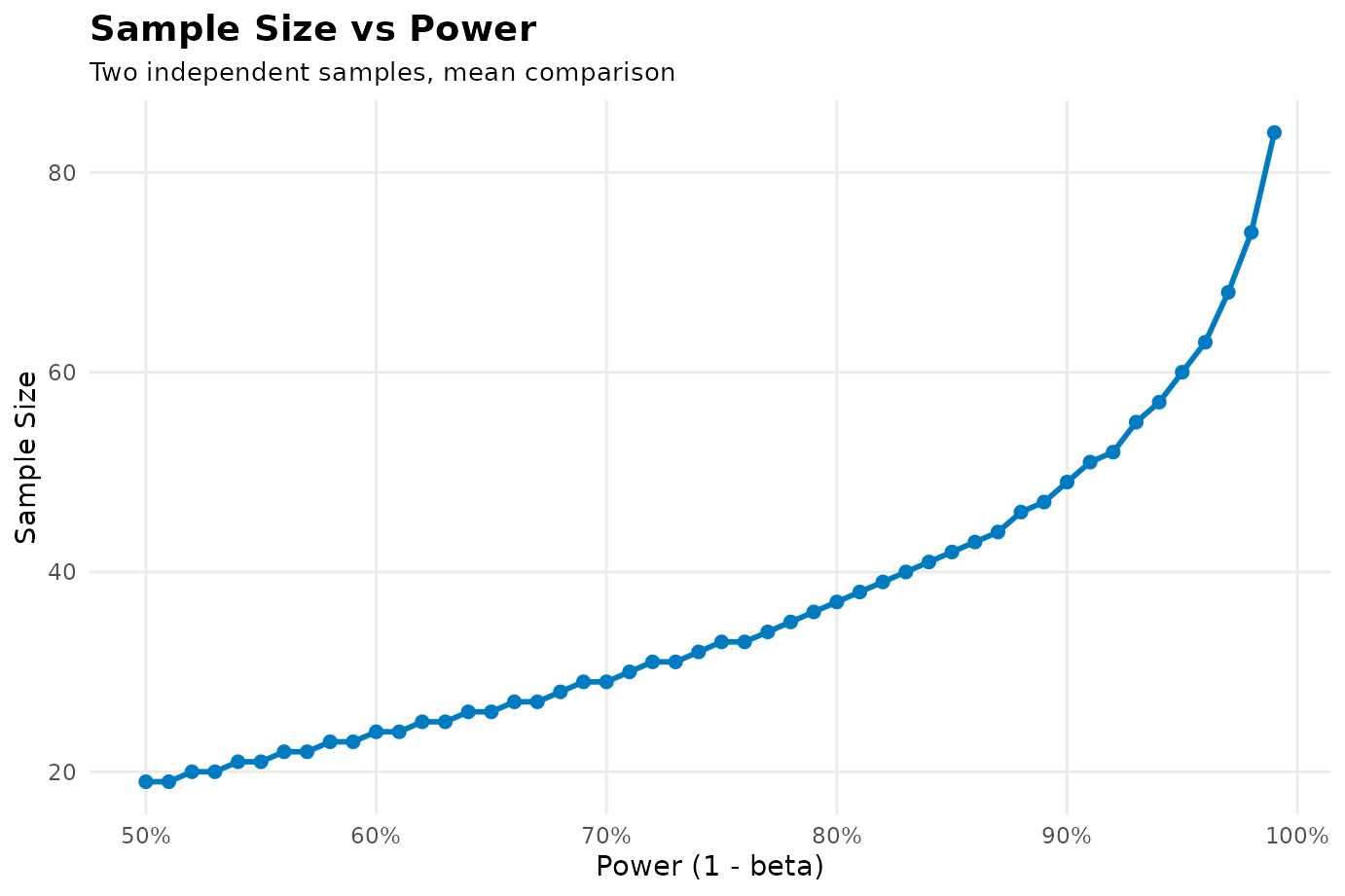

plot(res_1_1, type = "sample_size")

Portos (Yishan) Wang & AI Research Team

2026-11-04