Comprehensive Guide to sampleSizeCalc

Portos Wang (Yishan Wang), Bingxin Cai (Gansu Provincial Maternity and Child-care Hospital (Gansu Provincial Central Hospital))

2026-11-04

Introduction

The sampleSizeCalc package provides a comprehensive, rigorous toolkit for sample size determination across 39+ study design combinations in clinical and epidemiological research.

Looking for in-depth tutorials tailored for clinical researchers? - 📖 中文完全使用指南：临床科研样本量计算从入门到精通 (Comprehensive Guide in Chinese): 零基础入门，覆盖全部设计、参数白话解释、公式推导、生动临床案例、输出逐行精读与标书模板。 - 📘 English Comprehensive Guide (Zero-to-Hero Tutorial): End-to-end walkthrough covering all 39+ designs, intuitive statistical analogies, primary mathematical formulas, worked clinical scenarios, and protocol boilerplates.

The Three-Axis API (v3.0+)

The following examples are teaching protocols. Clinical rates, effects, SDs, and margins are illustrative inputs that need compatible evidence in a real study. The linked English and Chinese guides expand 52 scenarios with eligibility, endpoint timing, parameter rationale, and recruitment interpretation.

Scenario A — Antihypertensive RCT: Enroll adults with stable background treatment in a blinded, 1:1 parallel trial. Measure baseline-to-week-12 systolic BP reduction using standardized readings. Assume reductions of 10 and 12 mmHg and change-score SD 3 mmHg, with two-sided α=0.05 and 80% power. The SD concerns individual changes, and the result counts independent patients with complete endpoints.

calculate("rct", "test", "mean", mean1 = 10, mean2 = 12, sd = 3)
#> ────────────────────────────────────────────────────────────────────────────────
#> ✔ Sample Size Calculation Results
#> • Design type: "Two independent samples, mean comparison"
#> • Sample size per group: 37
#> • Total sample size: 74
#> Formula (plain text):
#> `n = 2 * ((Z_alpha/2 + Z_beta) * sd / (mean1 - mean2))^2`
#> Formula (LaTeX):
#> $$n = 2\left(\frac{Z_{\alpha/2} + Z_{\beta}}{\delta}\right)^2 = 2\left(\frac{(Z_{\alpha/2} + Z_{\beta}) \cdot \sigma}{\mu_1 - \mu_2}\right)^2$$
#> Calculation process:
#> 
#> • Step 1: State hypotheses: H0: mu1 = mu2 vs H1: mu1 != mu2 (two-sided alpha =
#> 0.05, power = 0.80).
#> • Step 2: Calculate mean difference delta = |mu1 - mu2| = |10 - 12| = 2; common
#> SD sigma = 3.
#> • Step 3: Determine critical values: Z_(alpha/2) = 1.96 (for two-sided alpha =
#> 0.05), Z_beta = 0.8416 (for power = 0.80).
#> • Step 4: Compute initial sample size via normal approximation: n0 = 2 *
#> ((Z_(alpha/2) + Z_beta) * sigma / delta)^2 = 2 * ((1.96 + 0.8416) * 3 / 2)^2 =
#> 35.32.
#> • Step 5: Refine via exact two-sample Student's t-test power iteration
#> (accounting for degrees of freedom df = 2n - 2).
#> • Step 6: Round up to integer: n = 37 per group, total sample size N = 74.
#> Reference:
#> Chow, S. C., Shao, J., Wang, H., & Lokhnygina, Y. (2017). Sample Size Calculations in Clinical Research (3rd ed.). CRC Press. Chapter 3 (Comparing Means), Section 3.2.1 two-sample parallel design, Eq 3.11 (p. 48; the Student t refinement is Table 3.2, p. 49).
#> 
#>  Also: Machin et al. (2018) Eq 5.4, p. 69 (same formula with the Student t correction term).
#> ────────────────────────────────────────────────────────────────────────────────
#> 

Scenario B — Prospective cardiovascular cohort: Recruit current smokers and never-smokers who are free of coronary disease at baseline, then ascertain the first prespecified event over 5 years using consistent follow-up. Assume cumulative risks of 30% and 20%, equal group sizes, and 10% loss to follow-up. These are fixed-period risks, not prevalence or rates per person-year; the returned count already includes the requested loss adjustment.

calculate("cohort", "test", "proportion", p0 = 0.20, p1 = 0.30, dropout = 0.10)
#> ────────────────────────────────────────────────────────────────────────────────
#> ✔ Sample Size Calculation Results
#> • Design type: "Cohort study (cumulative incidence, RR)"
#> • Sample size per group: 327
#> • Exposed group: 327
#> • Unexposed group: 327
#> • Total sample size: 654
#> Parameter roles
#> 
#> • p0 = unexposed-group cumulative incidence
#> • p1 = exposed-group cumulative incidence
#> • ratio = unexposed:exposed allocation (m)
#> • effect measure: risk ratio RR (estimable in cohort designs)
#> Formula (plain text):
#> `n1 = [Za*sqrt((1+1/m)*pbar*(1-pbar)) + Zb*sqrt(p1q1+p0q0/m)]^2/(p1-p0)^2`
#> Formula (LaTeX):
#> $$n_{1} = \frac{\left[Z_{\alpha/2}\sqrt{(1+\frac{1}{m})\bar{p}(1-\bar{p})} + Z_{\beta}\sqrt{p_1(1-p_1)+\frac{p_0(1-p_0)}{m}}\right]^2}{(p_1-p_0)^2}$$
#> Calculation process:
#> 
#> • Step 1: Specify proportions: unexposed p0 = 0.20, exposed p1 = 0.30,
#> allocation ratio m = 1 (alpha = 0.05, power = 0.80).
#> • Step 2: Weighted average proportion: p_bar = (p1 + m*p0) / (1 + m) = 0.25.
#> • Step 3: Determine critical values: Z_(alpha/2) = 1.96, Z_beta = 0.8416.
#> • Step 4: Calculate exposed sample size: n_exposed =
#> [Z_(alpha/2)*sqrt((1+1/m)*p_bar*(1-p_bar)) + Z_beta*sqrt(p1*q1 + p0*q0/m)]^2 /
#> (p1 - p0)^2 = 293.15.
#> • Step 5: Calculate unexposed sample size: n_unexposed = m * n_exposed = 1 *
#> 293.15 = 293.15.
#> • Step 6: Round up before dropout inflation: ceiling(n_exposed) = 294,
#> ceiling(m*n_exposed) = 294; apply dropout d = 0.10 using ceiling(n/(1-d)).
#> Exposed = 327, Unexposed = 327, Total sample size N = 654.
#> Reference:
#> Primary: Bhardwaj et al. (2024). Journal of Family Medicine and Primary Care, 13(7), 2559 (worked example: p0=0.20, p1=0.30, m=1 -> 293/group).
#> 
#>  Also: Schlesselman, J. J. (1982). Case-Control Studies. Oxford University Press (cohort/case-control shared formula, roles swapped); Machin et al. (2018) Ch.3.
#> ────────────────────────────────────────────────────────────────────────────────
#> 

Scenario C — Diagnostic ROC-AUC validation: Evaluate a frozen continuous biomarker score in reference-confirmed cases and clinically comparable non-cases, recruited in equal numbers. Each patient supplies one score and one reference result. Assume AUC 0.80 and a 95% CI half-width of 0.10 with a binormal variance model; the result must be met in both disease-status strata, not only as an overall total.

calculate("diagAUC", "estimate", "auc",
  auc = 0.80, d = 0.10,
  ratio = 1, var_method = "binormal"
)
#> ────────────────────────────────────────────────────────────────────────────────
#> ✔ Sample Size Calculation Results
#> • Design type: "Single-group AUC CI precision"
#> • Cases needed: 46
#> • Total subjects to screen: 92
#> • Total subjects: 92
#> Parameter roles
#> 
#> • auc = anticipated area under the ROC curve
#> • precision = desired CI half-width L
#> • ratio = case:control ratio R (cases:non-cases; default 1)
#> • var_method = binormal variance function
#> Formula (plain text):
#> `N_cases = (Z_1-a/2 / d)^2 * V(AUC)`
#> Formula (LaTeX):
#> $$n_{cases} = \left(\frac{Z_{1-\alpha/2}}{d}\right)^2 \cdot V(AUC)$$
#> Calculation process:
#> 
#> • Step 1: Anticipated AUC = 0.80, precision d = 0.10, supplied allocation R =
#> 1, alpha = 0.05.
#> • Step 2: Use the binormal variance model with the supplied allocation: V(AUC)
#> = 0.1195.
#> • Step 3: Calculate cases: n_cases = (Z_(1-alpha/2)/d)^2 * V(AUC) =
#> (1.96/0.10)^2 * 0.1195 = 45.89.
#> • Step 4: Convert using the supplied allocation: total = n_cases*(1+R) =
#> 45.89*(1+1) = 91.78.
#> • Step 5: Round up: Target cases needed = 46, Total subjects to screen = 92.
#> Reference:
#> Primary: Zhou, X.-H., Obuchowski, N. A., & McClish, D. K. (2011). Statistical Methods in Diagnostic Medicine (2nd ed.). Wiley. Section 6.1.2, pp. 196-199 (Eq 6.4/6.5/6.6; CTC worked example).
#> 
#>  Original variance: Hanley, J. A., & McNeil, B. J. (1982). Radiology, 143(1), 29-36.
#>  Binormal variance: Obuchowski, N. A. (1994). Computing sample size for receiver operating characteristic studies. Investigative Radiology, 29(2), 238-243.
#> ────────────────────────────────────────────────────────────────────────────────
#> 

Every result displays the plain-text formula, LaTeX source, calculation process, and literature references. Parameter roles (for example, p0 is unexposed incidence in a cohort but control-group exposure in a case-control study) and methodological hints are included where available. See the reporting guide for field extraction and a rendered formula example.

Introduction (legacy examples)

The sampleSizeCalc package provides a comprehensive toolkit for sample size determination in clinical research. It supports 17 different study designs across continuous outcomes, categorical outcomes, survival analysis, diagnostic accuracy, case-control studies, and AUC comparisons.

Key Features

• 17 Study Design Types with validated formulas
• Comprehensive Literature Support with primary methodology citations
• Robust Parameter Validation with clear error messages
• Modern S3 Methods (print, summary, plot)
• Flexible Output including sample sizes, event counts, and power curves

Installation

# Install from GitHub
devtools::install_github("portos-wang/Sample_Size_Calc")

# Or install from local source
devtools::install_local("path/to/1_sample_size_determination")

Continuous Outcomes

Two Independent Means (twoMeans)

Use case: Comparing means between two independent groups (e.g., treatment vs. control)

Example: A blinded outpatient trial compares baseline-to-week-12 systolic BP reductions under two add-on treatments. Assume group means of 10 and 12 mmHg and common change-score SD 3 mmHg. The two independent groups need complete patient-level change scores; repeated BP readings are averaged within the visit and are not separate patients.

result <- sample_size_calculator(
  design = "twoMeans",
  mean1 = 10, # Control group mean (mmHg reduction)
  mean2 = 12, # Treatment group mean (mmHg reduction)
  sd = 3, # Common standard deviation
  alpha = 0.05, # Significance level
  power = 0.8 # Target power (80%)
)

print(result)
#> ────────────────────────────────────────────────────────────────────────────────
#> ✔ Sample Size Calculation Results
#> • Design type: "Two independent samples, mean comparison"
#> • Sample size per group: 37
#> • Total sample size: 74
#> Formula (plain text):
#> `n = 2 * ((Z_alpha/2 + Z_beta) * sd / (mean1 - mean2))^2`
#> Formula (LaTeX):
#> $$n = 2\left(\frac{Z_{\alpha/2} + Z_{\beta}}{\delta}\right)^2 = 2\left(\frac{(Z_{\alpha/2} + Z_{\beta}) \cdot \sigma}{\mu_1 - \mu_2}\right)^2$$
#> Calculation process:
#> 
#> • Step 1: State hypotheses: H0: mu1 = mu2 vs H1: mu1 != mu2 (two-sided alpha =
#> 0.05, power = 0.80).
#> • Step 2: Calculate mean difference delta = |mu1 - mu2| = |10 - 12| = 2; common
#> SD sigma = 3.
#> • Step 3: Determine critical values: Z_(alpha/2) = 1.96 (for two-sided alpha =
#> 0.05), Z_beta = 0.8416 (for power = 0.80).
#> • Step 4: Compute initial sample size via normal approximation: n0 = 2 *
#> ((Z_(alpha/2) + Z_beta) * sigma / delta)^2 = 2 * ((1.96 + 0.8416) * 3 / 2)^2 =
#> 35.32.
#> • Step 5: Refine via exact two-sample Student's t-test power iteration
#> (accounting for degrees of freedom df = 2n - 2).
#> • Step 6: Round up to integer: n = 37 per group, total sample size N = 74.
#> Reference:
#> Chow, S. C., Shao, J., Wang, H., & Lokhnygina, Y. (2017). Sample Size Calculations in Clinical Research (3rd ed.). CRC Press. Chapter 3 (Comparing Means), Section 3.2.1 two-sample parallel design, Eq 3.11 (p. 48; the Student t refinement is Table 3.2, p. 49).
#> 
#>  Also: Machin et al. (2018) Eq 5.4, p. 69 (same formula with the Student t correction term).
#> ────────────────────────────────────────────────────────────────────────────────
#> 

Interpretation: - Need 37 subjects per group - Total sample size: 74 subjects - The effect size (Cohen’s d): 0.67

Formula: \[n = 2\left(\frac{(Z_{\alpha/2} + Z_{\beta}) \cdot \sigma}{\mu_1 - \mu_2}\right)^2\]

Reference: Chow et al. (2017). Sample Size Calculations in Clinical Research (3rd ed.). CRC Press.

---

Paired Means (pairedMeans)

Use case: Comparing means from paired or matched observations (e.g., pre-post measurements, matched pairs)

Example: A cognitive rehabilitation cohort receives the same prespecified cognitive assessment before and 12 weeks after training. Assume an average 2.5-point change and SD of patient-level differences 4.0 points, targeting 90% power. Both visits must be linked; practice effects and natural history require consideration when interpreting uncontrolled change.

result <- sample_size_calculator(
  design = "pairedMeans",
  meanDiff = 2.5, # Mean difference (post-pre)
  sdDiff = 4.0, # SD of differences
  alpha = 0.05,
  power = 0.9
)

print(result)
#> ────────────────────────────────────────────────────────────────────────────────
#> ✔ Sample Size Calculation Results
#> • Design type: "Paired means"
#> • Pairs needed: 29
#> • Total individuals: 58
#> Formula (plain text):
#> `n = ((Z_a/2 + Z_b) * sd_diff / mean_diff)^2`
#> Formula (LaTeX):
#> $$n = \left(\frac{(Z_{\alpha/2} + Z_{\beta}) \cdot \sigma_d}{\mu_d}\right)^2$$
#> Calculation process:
#> 
#> • Step 1: State paired difference hypotheses: H0: mu_d = 0 vs H1: mu_d != 0
#> (alpha = 0.05, power = 0.90).
#> • Step 2: Expected paired difference mu_d = 2.50, SD of differences sigma_d =
#> 4.
#> • Step 3: Determine critical values: Z_(alpha/2) = 1.96, Z_beta = 1.2816.
#> • Step 4: Normal approximation: n0 = ((Z_(alpha/2) + Z_beta) * sigma_d /
#> mu_d)^2 = ((1.96 + 1.2816) * 4 / 2.50)^2 = 26.90.
#> • Step 5: Exact paired Student's t-test degrees of freedom iteration.
#> • Step 6: Round up to integer: n = 29 pairs (total individuals = 58).
#> Reference:
#> Rosner, B. (2015). *Fundamentals of biostatistics* (8th ed.). Cengage Learning.
#> ────────────────────────────────────────────────────────────────────────────────
#> 

Interpretation: - Need 29 pairs (i.e., 58 measurements from 29 subjects) - Standardized effect size: 0.62

Reference: Rosner (2015). Fundamentals of Biostatistics (8th ed.). Cengage Learning.

---

Categorical Outcomes

Two Proportions (twoProportions)

Use case: Comparing proportions between two independent groups

Example: An exploratory oncology trial compares objective response at a fixed week-12 assessment, using the same imaging criteria in both randomized groups. Assume response rates of 30% and 45%, with two-sided α=0.05 and 80% power. Prespecify early deaths, rescue therapy, and unevaluable imaging rather than excluding unsuccessful patients from the denominator.

result <- sample_size_calculator(
  design = "twoProportions",
  p1 = 0.30, # Control response rate
  p2 = 0.45, # Treatment response rate
  alpha = 0.05,
  power = 0.8
)

print(result)
#> ────────────────────────────────────────────────────────────────────────────────
#> ✔ Sample Size Calculation Results
#> • Design type: "Two independent proportions"
#> • Sample size per group: 163
#> • Total sample size: 326
#> Formula (plain text):
#> `n = (Z_a/2 * sqrt(2*p_bar*(1-p_bar)) + Z_b * sqrt(p1*(1-p1)+p2*(1-p2)))^2 /
#> (p1-p2)^2`
#> Formula (LaTeX):
#> $$n = \frac{\left[Z_{\alpha/2}\sqrt{2\bar{p}(1-\bar{p})} + Z_{\beta}\sqrt{p_1(1-p_1) + p_2(1-p_2)}\right]^2}{(p_1 - p_2)^2}$$
#> Calculation process:
#> 
#> • Step 1: State hypotheses: H0: p1 = p2 vs H1: p1 != p2 (two-sided alpha =
#> 0.05, power = 0.80).
#> • Step 2: Compute pooled proportion: p_bar = (p1 + p2) / 2 = (0.30 + 0.45) / 2
#> = 0.375.
#> • Step 3: Determine critical values: Z_(alpha/2) = 1.96, Z_beta = 0.8416.
#> • Step 4: Compute Fleiss formula numerator components:
#> Z_(alpha/2)*sqrt(2*p_bar*(1-p_bar)) = 1.3419; Z_beta*sqrt(p1(1-p1)+p2(1-p2)) =
#> 0.5693.
#> • Step 5: Calculate unrounded sample size per group: n = (1.3419 + 0.5693)^2 /
#> (0.30 - 0.45)^2 = 162.33.
#> • Step 6: Round up to integer: n = 163 per group, total sample size N = 326.
#> Reference:
#> Primary (formula as implemented, without continuity correction): Fleiss, J. L., Tytun, A., & Ury, H. K. (1980). A simple approximation for calculating sample sizes for comparing independent proportions. Biometrics, 36(2), 343-346.
#> 
#> With continuity correction: Casagrande, J. T., Pike, M. C., & Smith, P. G. (1978). An improved approximate formula for calculating sample sizes for comparing two binomial distributions. Biometrics, 34(3), 483-494.
#> 
#> Book: Fleiss, J. L., Levin, B., & Paik, M. C. (2003). Statistical methods for rates and proportions (3rd ed.). Wiley.
#> ────────────────────────────────────────────────────────────────────────────────
#> 

Interpretation: - Need 163 patients per group - Absolute risk reduction: 0.15 - Relative risk increase: 50%

Reference: Fleiss et al. (2003). Statistical Methods for Rates and Proportions (3rd ed.). Wiley.

---

Survival Analysis

Survival (Log-rank Test, survival)

Use case: Time-to-event analysis with log-rank test

Example: A randomized oncology trial uses all-cause death from randomization as the overall-survival endpoint, with last-known survival as the censoring date. Assume HR 0.70 under proportional hazards and 1:1 allocation. First calculate deaths required, then use accrual and survival assumptions to estimate patient enrollment and follow-up duration.

result <- sample_size_calculator(
  design = "survival",
  hr = 0.70, # Hazard ratio (treatment vs. control)
  pE = 0.50, # Proportion in experimental group (1:1 randomization)
  alpha = 0.05,
  power = 0.8
)

print(result)
#> ────────────────────────────────────────────────────────────────────────────────
#> ✔ Sample Size Calculation Results
#> • Design type: "Survival (log-rank)"
#> • Events needed: 247
#> Formula (plain text):
#> `E = (Z_a/2 + Z_b)^2 / (pE*(1-pE)*log(HR)^2)`
#> Formula (LaTeX):
#> $$E = \frac{(Z_{\alpha/2} + Z_{\beta})^2}{p_E(1-p_E)[\ln(HR)]^2}$$
#> Calculation process:
#> 
#> • Step 1: State survival parameters: Hazard Ratio HR = 0.70, experimental arm
#> allocation pE = 0.50 (alpha = 0.05, power = 0.80).
#> • Step 2: Compute log hazard ratio: ln(HR) = ln(0.70) = -0.3567.
#> • Step 3: Determine critical values: Z_(alpha/2) = 1.96, Z_beta = 0.8416.
#> • Step 4: Apply Schoenfeld formula: E = (Z_(alpha/2) + Z_beta)^2 / [pE * (1 -
#> pE) * (ln HR)^2] = (1.96 + 0.8416)^2 / [0.50 * 0.50 * (-0.3567)^2] = 246.79.
#> • Step 5: Round up to integer: Target events needed E = 247.
#> Reference:
#> Primary: Schoenfeld, D. A. (1983). Sample-size formula for the proportional-hazards regression model. Biometrics, 39(2), 499-503.
#> 
#> Extensions:
#> - Hsieh, F. Y., & Lavori, P. W. (2000). Sample-size calculations for the Cox proportional hazards regression model with nonbinary covariates. Controlled Clinical Trials, 21(6), 552-560.
#> - Rubinstein, L. V., Gail, M. H., & Santner, T. J. (1981). Planning the duration of a comparative clinical trial with loss to follow-up and a period of continued observation. Journal of Chronic Diseases, 34(9-10), 469-479.
#> ────────────────────────────────────────────────────────────────────────────────
#> 

Important Notes: - This calculates the number of events needed, not the total sample size - Total sample size = events / event rate - For example, if event rate is 50%, total sample size needed: 494 subjects

Formula: \[E = \frac{(Z_{\alpha/2} + Z_{\beta})^2}{p_E(1-p_E)[\ln(HR)]^2}\]

Reference: Schoenfeld (1983). Sample-size formula for the proportional-hazards regression model. Biometrics, 39(2), 499-503.

---

Non-Inferiority, Superiority, and Equivalence

Non-Inferiority Test (Means, nonInferiorityMeans)

Use case: Demonstrating that a new treatment is not worse than standard by more than a margin

Example: A parallel trial evaluates whether a simpler symptom-management strategy preserves most of an active comparator’s improvement on a prespecified depression score at week 12. Assume mean improvements 8.0 versus 8.5 points, SD 2.0, and maximum acceptable loss 1.0 point. Use one-sided α=0.025 and 90% power; the margin needs its own clinical and effect-preservation justification.

result <- sample_size_calculator(
  design = "nonInferiorityMeans",
  mean1 = 8.0, # New treatment mean
  mean2 = 8.5, # Standard treatment mean
  sd = 2.0, # Common SD
  margin = 1.0, # Non-inferiority margin (Δ)
  alpha = 0.025, # One-sided test
  power = 0.9
)

print(result)
#> ────────────────────────────────────────────────────────────────────────────────
#> ✔ Sample Size Calculation Results
#> • Design type: "Non-inferiority (means)"
#> • Sample size per group: 337
#> • Total sample size: 674
#> Formula (plain text):
#> `n = 2*(Z_a+Z_b)^2*sd^2/(mean1-mean2+margin)^2`
#> Formula (LaTeX):
#> $$n = 2\left(\frac{(Z_{\alpha} + Z_{\beta})\sigma}{\mu_1 - \mu_2 + \Delta}\right)^2$$
#> Calculation process:
#> 
#> • Step 1: State non-inferiority hypotheses: H0: mu1 - mu2 <= -margin vs H1: mu1
#> - mu2 > -margin (margin Delta = 1, one-sided alpha = 0.025, power = 0.90).
#> • Step 2: Effective difference: delta_E = mu1 - mu2 + margin = 8 - 8.50 + 1 =
#> 0.50; SD sigma = 2.
#> • Step 3: Determine critical values: one-sided Z_alpha = 1.96, Z_beta = 1.2816.
#> • Step 4: Compute sample size: n = 2 * (Z_alpha + Z_beta)^2 * sigma^2 /
#> delta_E^2 = 2 * (1.96 + 1.2816)^2 * 2^2 / (0.50)^2 = 336.24.
#> • Step 5: Round up to integer: n = 337 per group, total sample size N = 674.
#> Reference:
#> Chow, S. C., Shao, J., Wang, H., & Lokhnygina, Y. (2017). Sample Size Calculations in Clinical Research (3rd ed.). CRC Press. Chapter 3 (Comparing Means), Section 3.2.2 noninferiority, Eq 3.12, p. 50.
#> 
#>  Also: Machin et al. (2018) Eq 11.3, p. 173.
#> ────────────────────────────────────────────────────────────────────────────────
#> 

Key Points: - Uses one-sided α (typically 0.025) - Margin Δ defines clinically acceptable difference - New treatment must be within Δ of standard

Reference: Chow et al. (2017). Sample Size Calculations in Clinical Research (3rd ed.). CRC Press.

---

Superiority Test (Means, superiorityMeans)

Use case: Demonstrating that a new treatment is better than standard

Example: A pain trial compares week-12 improvement on a specified 0–100 scale, assuming means of 12 and 10 points and SD 2.5. The objective is to exceed the active comparator by more than 0.5 point, using one-sided α=0.025 and 85% power. The effective difference in the formula is the anticipated difference minus that prespecified superiority margin.

result <- sample_size_calculator(
  design = "superiorityMeans",
  mean1 = 12.0, # New treatment mean (better)
  mean2 = 10.0, # Standard treatment mean
  sd = 2.5, # Common SD
  margin = 0.5, # Minimal clinically important difference
  alpha = 0.025, # One-sided test
  power = 0.85
)

print(result)
#> ────────────────────────────────────────────────────────────────────────────────
#> ✔ Sample Size Calculation Results
#> • Design type: "Superiority (means)"
#> • Sample size per group: 50
#> • Total sample size: 100
#> Formula (plain text):
#> `n = 2*(Z_a+Z_b)^2*sd^2/(mean1-mean2-margin)^2`
#> Formula (LaTeX):
#> $$n = 2\left(\frac{(Z_{\alpha} + Z_{\beta})\sigma}{\mu_1 - \mu_2 - \Delta}\right)^2$$
#> Calculation process:
#> 
#> • Step 1: State superiority hypotheses: H0: mu1 - mu2 <= margin vs H1: mu1 -
#> mu2 > margin (margin Delta = 0.50, one-sided alpha = 0.025, power = 0.85).
#> • Step 2: Effective difference: delta_E = mu1 - mu2 - margin = 12 - 10 - 0.50 =
#> 1.50; SD sigma = 2.50.
#> • Step 3: Determine critical values: one-sided Z_alpha = 1.96, Z_beta = 1.0364.
#> • Step 4: Compute sample size: n = 2 * (Z_alpha + Z_beta)^2 * sigma^2 /
#> delta_E^2 = 2 * (1.96 + 1.0364)^2 * 2.50^2 / (1.50)^2 = 49.88.
#> • Step 5: Round up to integer: n = 50 per group, total sample size N = 100.
#> Reference:
#> Chow, S. C., Shao, J., Wang, H., & Lokhnygina, Y. (2017). Sample Size Calculations in Clinical Research (3rd ed.). CRC Press. Chapter 3 (Comparing Means), Section 3.2.2 superiority, Eq 3.12, p. 50.
#> 
#>  Also: Machin et al. (2018) Eq 11.3, p. 173.
#> ────────────────────────────────────────────────────────────────────────────────
#> 

Key Points: - Uses one-sided α - Effect must exceed margin to be meaningful - Smaller margin requires larger sample size

---

Equivalence Test (Means, equivalenceMeans)

Use case: Demonstrating two treatments are equivalent

Example: Two randomized anemia-support strategies are compared on mean hemoglobin at week 12, assuming 100 versus 102 g/L and SD 5 g/L. The teaching equivalence interval is ±5 g/L, with one-sided α=0.05 and 80% power. This is equivalence of a specified continuous endpoint, distinct from a pharmacokinetic bioequivalence study.

result <- sample_size_calculator(
  design = "equivalenceMeans",
  mean1 = 100, # Test mean
  mean2 = 102, # Reference mean
  sd = 5, # Common SD
  margin = 5, # Equivalence margin (±5 units)
  alpha = 0.05,
  power = 0.8
)

print(result)
#> ────────────────────────────────────────────────────────────────────────────────
#> ✔ Sample Size Calculation Results
#> • Design type: "Equivalence (means)"
#> • Sample size per group: 48
#> • Total sample size: 96
#> Formula (plain text):
#> `n = 2*(Z_a+Z_b/2)^2*sd^2/(margin-|mean1-mean2|)^2`
#> Formula (LaTeX):
#> $$n = 2\left(\frac{(Z_{\alpha} + Z_{\beta/2})\sigma}{\Delta - |\mu_1 - \mu_2|}\right)^2$$
#> Calculation process:
#> 
#> • Step 1: State equivalence hypotheses (TOST): H0: |mu1 - mu2| >= margin vs H1:
#> |mu1 - mu2| < margin (margin Delta = 5, alpha = 0.05, power = 0.80).
#> • Step 2: Margin clearance: Delta - |mu1 - mu2| = 5 - |100 - 102| = 3; SD sigma
#> = 5.
#> • Step 3: Determine critical values: one-sided Z_alpha = 1.6449, Z_(beta/2) =
#> 1.2816.
#> • Step 4: Compute sample size: n = 2 * (Z_alpha + Z_(beta/2))^2 * sigma^2 /
#> (Delta - |mu1 - mu2|)^2 = 2 * (1.6449 + 1.2816)^2 * 5^2 / (3)^2 = 47.58.
#> • Step 5: Round up to integer: n = 48 per group, total sample size N = 96.
#> Reference:
#> Chow, S. C., Shao, J., Wang, H., & Lokhnygina, Y. (2017). Sample Size Calculations in Clinical Research (3rd ed.). CRC Press. Chapter 3 (Comparing Means), Section 3.2.3 equivalence, Eq 3.13, p. 51; the Z_{beta/2} convention is discussed in Section 3.6.1 (p. 67).
#> 
#>  Also: Machin et al. (2018) Eq 11.5-11.6, p. 174.
#> ────────────────────────────────────────────────────────────────────────────────
#> 

Key Points: - Uses TOST (Two One-Sided Tests) procedure - Requires Z_β/2 (larger sample size) - Margin must be larger than observed difference

---

Diagnostic Accuracy Studies

Diagnostic Accuracy (Single Test, diagnosticAccuracySingle)

Use case: Estimating sensitivity or specificity with a given precision

Example: A referral clinic consecutively validates a locked-threshold diagnostic test using a common reference examination for all patients. Assume sensitivity 85%, 95% CI half-width 0.05, and source prevalence 20%. The case requirement is confirmed disease-positive patients; total screening is an expectation-based conversion, and specificity precision requires separate planning.

result <- sample_size_calculator(
  design = "diagnosticAccuracySingle",
  prob = 0.85, # Expected sensitivity
  d = 0.05, # Desired precision (±5%)
  prevalence = 0.20, # Disease prevalence
  alpha = 0.05
)

print(result)
#> ────────────────────────────────────────────────────────────────────────────────
#> ✔ Sample Size Calculation Results
#> • Design type: "Diagnostic accuracy (single)"
#> • Cases needed: 196
#> • Total subjects to screen: 980
#> Formula (plain text):
#> `N_cases = (Z_1-a/2)^2 * P*(1-P)/d^2`
#> Formula (LaTeX):
#> $$n_{{{cases}}} = \frac{Z_{1-\alpha/2}^2 \cdot p(1-p)}{d^2}$$
#> Calculation process:
#> 
#> • Step 1: Specify diagnostic accuracy prob (Se or Sp) = 0.85, margin of error d
#> = 0.05, prevalence = 0.20 (alpha = 0.05).
#> • Step 2: Determine critical value: Z_(1-alpha/2) = 1.96 (confidence level =
#> 95%).
#> • Step 3: Calculate target cases required: n_cases = Z_sum^2 * prob * (1 -
#> prob) / d^2 = (1.96)^2 * 0.85 * 0.15 / (0.05)^2 = 195.91.
#> • Step 4: Adjust for disease prevalence: total subjects to screen = n_cases /
#> prevalence = 195.91 / 0.20 = 979.57.
#> • Step 5: Round up to integer: Target cases needed = 196, Total subjects to
#> screen = 980.
#> Reference:
#> Primary: Hanley, J. A., & McNeil, B. J. (1982). The meaning and use of the area under a receiver operating characteristic (ROC) curve. Radiology, 143(1), 29-36.
#> 
#> Review: Hajian-Tilaki, K. (2014). Sample size estimation in diagnostic test studies of biomedical informatics. Journal of Biomedical Informatics, 48, 193-204.
#> ────────────────────────────────────────────────────────────────────────────────
#> 

Interpretation: - Target state cases needed: 196 - Total subjects to screen: 980 - With 20% prevalence, need to screen 980 to get 196 cases

Formula: \[n_{cases} = \frac{Z_{1-\alpha/2}^2 \cdot p(1-p)}{d^2}\]

Reference: Hajian-Tilaki (2014). Sample size determination in diagnostic test studies. Journal of Biomedical Informatics, 48, 193-204.

---

AUC (Single Group, auc_single)

Use case: Estimating AUC with a confidence interval of given width

Example: A biomarker score is frozen before a clinical validation cohort is enrolled. Assume AUC 0.80, CI half-width 0.05, and source prevalence 30%, with one score and a reference disease assessment per person. This legacy branch uses its Hanley–McNeil variance calculation; the three-axis example above demonstrates explicitly selecting a different variance model.

result <- sample_size_calculator(
  design = "auc_single",
  auc = 0.80, # Expected AUC
  d = 0.05, # Half-width of CI (±0.10 total)
  prevalence = 0.30,
  alpha = 0.05
)

print(result)
#> ────────────────────────────────────────────────────────────────────────────────
#> ✔ Sample Size Calculation Results
#> • Design type: "Single-group AUC CI precision"
#> • Cases needed: 144
#> • Total subjects to screen: 478
#> Formula (plain text):
#> `N_cases = (Z_1-a/2 / d)^2 * V(AUC), V = 0.0099*exp(-a^2/2)*([5a^2+8] +
#> [a^2+8]/R), a = qnorm(A)*1.414`
#> Formula (LaTeX):
#> $$n_{cases} = \left(\frac{Z_{1-\alpha/2}}{d}\right)^2 \cdot \left\{0.0099\,e^{-a^2/2}\left([5a^2+8]+\frac{a^2+8}{R}\right)\right\}, \quad a = \Phi^{-1}(A)\cdot 1.414$$
#> Calculation process:
#> 
#> • Step 1: Specify anticipated AUC = 0.80, desired precision d = 0.05,
#> prevalence = 0.30 (alpha = 0.05).
#> • Step 2: Hanley-McNeil variance components: Q1 = AUC/(2-AUC) = 0.6667, Q2 =
#> 2*AUC^2/(1+AUC) = 0.7111.
#> • Step 3: Compute variance factor: V(AUC) = 0.2425.
#> • Step 4: Calculate cases needed: n_cases = (Z_(1-alpha/2) / d)^2 * V(AUC) =
#> (1.96 / 0.05)^2 * 0.2425 = 372.68.
#> • Step 5: Adjust for prevalence: screening total = n_cases / prevalence =
#> 372.68 / 0.30 = 1242.27.
#> • Step 6: Round up to integer: Target cases needed = 144, Total subjects to
#> screen = 478.
#> Reference:
#> Primary: Zhou, X.-H., Obuchowski, N. A., & McClish, D. K. (2011). Statistical Methods in Diagnostic Medicine (2nd ed.). Wiley. Section 6.1.2, Eq 6.5, pp. 196-198 (binormal variance function).
#> 
#>  Variance function: Obuchowski, N. A. (1994). Computing sample size for receiver operating characteristic studies. Investigative Radiology, 29(2), 238-243.
#> 
#>  Review: Hajian-Tilaki, K. (2014). Journal of Biomedical Informatics, 48, 193-204 (Eq 7.4).
#> ────────────────────────────────────────────────────────────────────────────────
#> 

Key Points: - Calculates cases with disease - AUC variance depends on AUC value and prevalence - Hanley-McNeil method is standard approach

Reference: Hanley & McNeil (1982). The meaning and use of AUC. Radiology, 143(1), 29-36.

---

AUC Comparison (Two Tests, aucComparison)

Use case: Comparing AUCs of two diagnostic tests applied to same subjects

Example: The same patients receive two continuous imaging scores, each evaluated against one common disease reference. Assume AUCs 0.85 and 0.80, correlation between the AUC estimators 0.6, and prevalence 25%. Preserve pairing and use pilot covariance information; correlation between raw image scores is not automatically the required AUC correlation.

result <- sample_size_calculator(
  design = "aucComparison",
  auc1 = 0.85, # Test 1 AUC
  auc2 = 0.80, # Test 2 AUC
  r = 0.6, # Correlation between AUCs
  prevalence = 0.25,
  alpha = 0.05,
  power = 0.8
)

print(result)
#> ────────────────────────────────────────────────────────────────────────────────
#> ✔ Sample Size Calculation Results
#> • Design type: "AUC comparison (two tests)"
#> • Cases needed: 208
#> • Total subjects to screen: 830
#> Formula (plain text):
#> `n_cases = 2 * (Z_alpha/2 + Z_beta)^2 * V(AUC) * (1 - r) / (AUC1 - AUC2)^2,
#> binormal V`
#> Formula (LaTeX):
#> $$n_{cases} = \frac{2(Z_{\alpha/2} + Z_{\beta})^2 \cdot V(AUC) \cdot (1-r)}{(AUC_1 - AUC_2)^2}$$
#> Calculation process:
#> 
#> • Step 1: Specify AUC1 = 0.85, AUC2 = 0.80, correlation r = 0.60, prevalence =
#> 0.25 (alpha = 0.05, power = 0.80).
#> • Step 2: Determine critical values: Z_(alpha/2) = 1.96, Z_beta = 0.8416.
#> • Step 3: Evaluate pooled Hanley-McNeil variance V(AUC_avg).
#> • Step 4: Calculate target cases: n_cases = 2 * (Z_(alpha/2) + Z_beta)^2 *
#> V(AUC) * (1 - r) / (AUC1 - AUC2)^2.
#> • Step 5: Round up to integer: Target cases needed = 208, Total subjects to
#> screen = 830.
#> Reference:
#> Primary: Hajian-Tilaki, K. (2014). Sample size estimation in diagnostic test studies of biomedical informatics. Journal of Biomedical Informatics, 48, 193-204 (Eq 7.6-7.8, paired/independent two-AUC comparison; the worked example on p. 199 gives n = 211 with the binormal variance). https://doi.org/10.1016/j.jbi.2014.02.013
#> 
#>  Variance function: Zhou, X.-H., Obuchowski, N. A., & McClish, D. K. (2011). Statistical Methods in Diagnostic Medicine (2nd ed.), Eq 6.5.
#> ────────────────────────────────────────────────────────────────────────────────
#> 

Key Points: - Requires correlation coefficient (r) - Higher correlation → smaller sample size - Uses Hanley-McNeil method for paired design

---

Case-Control Studies

Case-Control (caseControl)

Use case: Sample size for case-control studies with odds ratio

Example: Incident lung cancer cases and controls from the same source population report smoking before a common index-date window. Assume 30% control exposure and OR 2.5, with one control per case. This is an unmatched group-ratio design; p0 is exposure prevalence among controls, and individual age matching would require a different calculation.

result <- sample_size_calculator(
  design = "caseControl",
  p0 = 0.30, # Exposure rate in controls
  OR = 2.5, # Target odds ratio
  m = 1, # Controls per case (unmatched group ratio)
  alpha = 0.05,
  power = 0.8
)

print(result)
#> ────────────────────────────────────────────────────────────────────────────────
#> ✔ Sample Size Calculation Results
#> • Design type: "Case-control"
#> • Cases needed: 80
#> • Controls needed: 80
#> • Total subjects: 160
#> Formula (plain text):
#> `n_cases = [Z_alpha/2 * sqrt((1+1/m)*p_bar*(1-p_bar)) + Z_beta * sqrt(p1*(1-p1)
#> + p0*(1-p0)/m)]^2 / (p1 - p0)^2`
#> Formula (LaTeX):
#> $$n_{cases} = \frac{\left[Z_{\alpha/2}\sqrt{(1+1/m)\bar{p}(1-\bar{p})} + Z_{\beta}\sqrt{p_1(1-p_1) + p_0(1-p_0)/m}\right]^2}{(p_1-p_0)^2}$$
#> Calculation process:
#> 
#> • Step 1: Compute case exposure rate from Odds Ratio: p1 = (OR * p0) / (1 - p0
#> + OR * p0) = (2.50 * 0.30) / (1 - 0.30 + 2.50 * 0.30) = 0.5172.
#> • Step 2: Weighted average exposure (matching ratio m = 1): p_bar = (p1 + m*p0)
#> / (1 + m) = 0.4086.
#> • Step 3: Determine critical values: Z_(alpha/2) = 1.96, Z_beta = 0.8416.
#> • Step 4: Schlesselman formula for cases: n_cases =
#> [Z_(alpha/2)*sqrt((1+1/m)*p_bar*(1-p_bar)) + Z_beta*sqrt(p1*(1-p1) +
#> p0*(1-p0)/m)]^2 / (p1 - p0)^2 = 79.19.
#> • Step 5: Calculate controls needed: n_controls = m * n_cases = 1 * 79.19 =
#> 79.19.
#> • Step 6: Round up to integer: Cases needed = 80, Controls needed = 80, Total
#> subjects = 160.
#> Reference:
#> Primary: Schlesselman, J. J. (1982). Case-control studies: Design, conduct, analysis. Oxford University Press.
#> 
#> IARC classic: Breslow, N. E., & Day, N. E. (1980). Statistical methods in cancer research: Volume I - The analysis of case-control studies. IARC Scientific Publications No. 32.
#> 
#> For individually matched designs (not the formula implemented here): Dupont, W. D. (1988). Power calculations for matched case-control studies. Biometrics, 44(4), 1157-1168; see the caseControlMatched design.
#> ────────────────────────────────────────────────────────────────────────────────
#> 

Interpretation: - Cases needed: 80 - Controls needed: 80 - Total subjects: 160

Reference: Schlesselman (1982). Case-Control Studies: Design, Conduct, Analysis. Oxford University Press.

---

Advanced Usage

Plotting Power Curves

The plot() method can visualize power curves:

result <- sample_size_calculator(
  "twoMeans",
  mean1 = 10,
  mean2 = 12,
  sd = 3,
  alpha = 0.05,
  power = 0.8
)

# Plot sample size vs. power
plot(result, type = "power")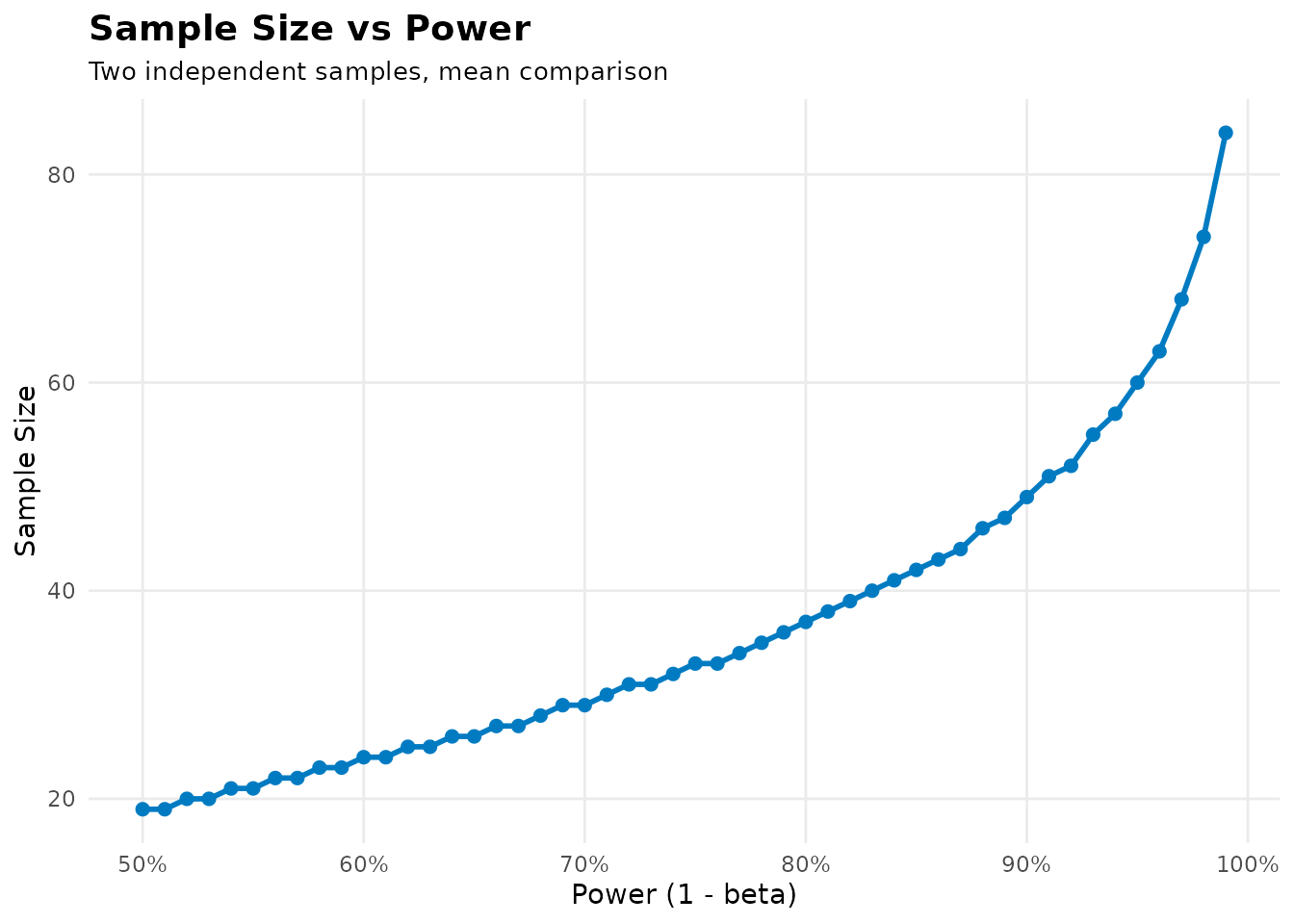

Plotting Sample Size vs. Effect Size

# Plot sample size vs. effect size ratio
plot(result, type = "sample_size")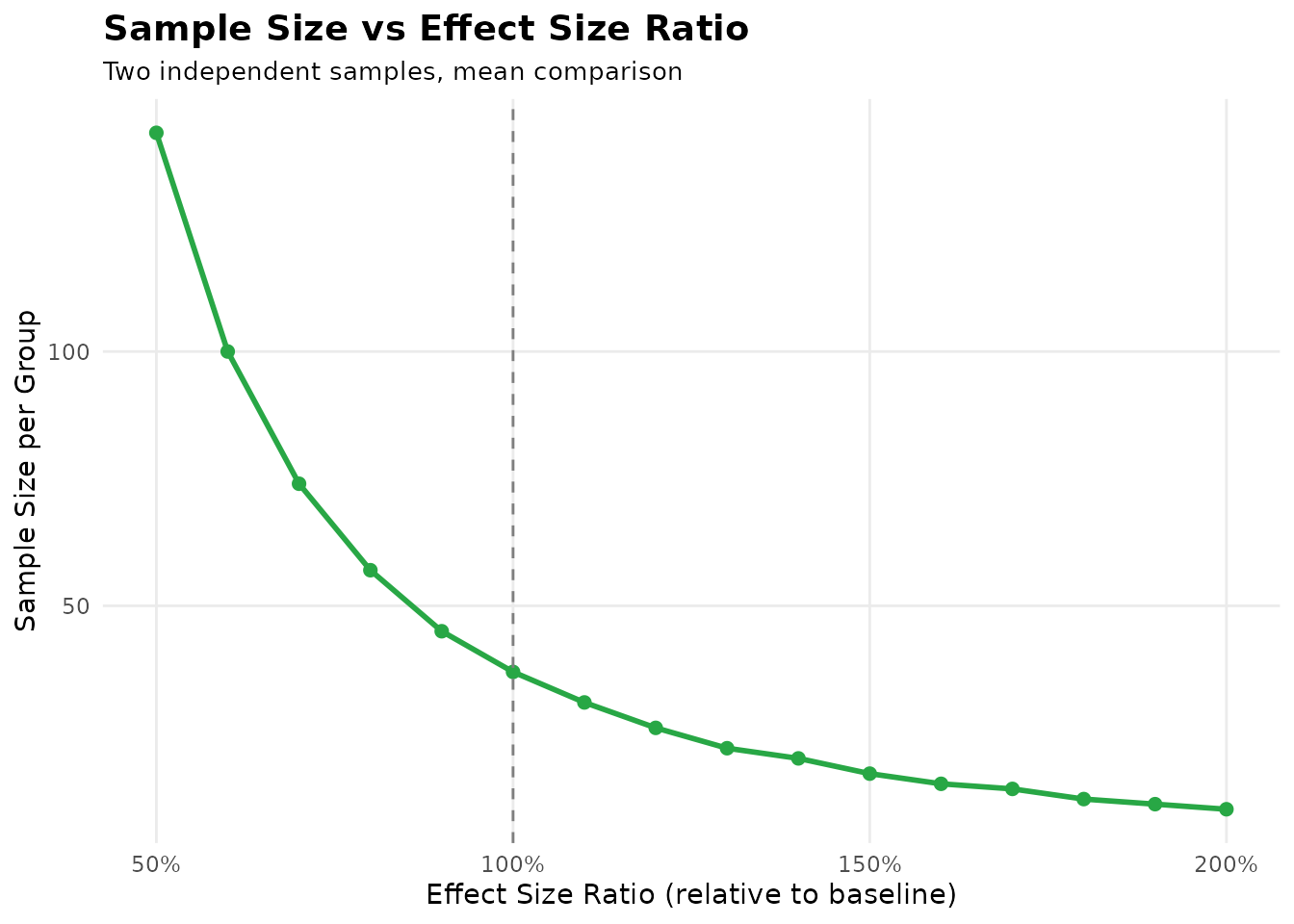

Using summary() for Parameters and Adjustments

Default print() output already includes the four report components. summary() expands the report with all input parameters, design axes where available, and recorded adjustments.

result <- sample_size_calculator(
  "survival",
  hr = 0.70,
  alpha = 0.05,
  power = 0.8
)

summary(result)
#> ────────────────────────────────────────────────────────────────────────────────
#> ✔ Sample Size Calculation Summary
#> ────────────────────────────────────────────────────────────────────────────────
#> 
#> ── Study Design
#> • Type: "Survival (log-rank)"
#> 
#> ── Parameters
#> • hazard_ratio: 0.7
#> • allocation_ratio: 0.5
#> • alpha: 0.05
#> • power: 0.8
#> 
#> ── Sample Size Results
#> • Events needed: 247
#> 
#> ── Formula
#> Plain text:
#> `E = (Z_a/2 + Z_b)^2 / (pE*(1-pE)*log(HR)^2)`
#> LaTeX:
#> $$E = \frac{(Z_{\alpha/2} + Z_{\beta})^2}{p_E(1-p_E)[\ln(HR)]^2}$$
#> 
#> ── Calculation Process
#> • Step 1: State survival parameters: Hazard Ratio HR = 0.70, experimental arm
#> allocation pE = 0.50 (alpha = 0.05, power = 0.80).
#> • Step 2: Compute log hazard ratio: ln(HR) = ln(0.70) = -0.3567.
#> • Step 3: Determine critical values: Z_(alpha/2) = 1.96, Z_beta = 0.8416.
#> • Step 4: Apply Schoenfeld formula: E = (Z_(alpha/2) + Z_beta)^2 / [pE * (1 -
#> pE) * (ln HR)^2] = (1.96 + 0.8416)^2 / [0.50 * 0.50 * (-0.3567)^2] = 246.79.
#> • Step 5: Round up to integer: Target events needed E = 247.
#> 
#> ── Reference
#> Primary: Schoenfeld, D. A. (1983). Sample-size formula for the proportional-hazards regression model. Biometrics, 39(2), 499-503.
#> 
#> Extensions:
#> - Hsieh, F. Y., & Lavori, P. W. (2000). Sample-size calculations for the Cox proportional hazards regression model with nonbinary covariates. Controlled Clinical Trials, 21(6), 552-560.
#> - Rubinstein, L. V., Gail, M. H., & Santner, T. J. (1981). Planning the duration of a comparative clinical trial with loss to follow-up and a period of continued observation. Journal of Chronic Diseases, 34(9-10), 469-479.
#> ────────────────────────────────────────────────────────────────────────────────

The summary includes:

• Study design description
• All parameters used
• Sample size results
• Formula in plain text and LaTeX source
• Calculation process
• Literature references
• Parameter roles and recorded adjustments where available

Extracting the Report Components

result$formula
cat(result$formula_latex)
cat(result$calculation_steps, sep = "\n")
cat(result$reference)

calculation is an alias for calculation_steps. Both the three-axis API and sample_size_calculator() provide these report fields.

---

Best Practices

1. Estimate Effect Sizes from Prior Studies

# DON'T: Use unrealistic effect sizes
sample_size_calculator("twoMeans", mean1 = 10, mean2 = 15, sd = 3)

# DO: Use effect sizes from literature or pilot studies
# From meta-analysis: standardized mean difference = 0.5
smd <- 0.5
sd <- 3
mean_diff <- smd * sd # 1.5
sample_size_calculator("twoMeans", mean1 = 10, mean2 = 10 + mean_diff, sd = sd)

2. Adjust for Dropout

# Calculate required sample size
result <- sample_size_calculator("twoMeans", mean1 = 10, mean2 = 12, sd = 3, power = 0.8)
n_per_group <- result$n_per_group

# Adjust for 20% dropout
dropout_rate <- 0.20
n_adjusted <- ceiling(n_per_group / (1 - dropout_rate))

3. Consider Multiple Scenarios

# Conservative scenario (smaller effect)
result1 <- sample_size_calculator("twoMeans", mean1 = 10, mean2 = 11, sd = 3)

# Optimistic scenario (larger effect)
result2 <- sample_size_calculator("twoMeans", mean1 = 10, mean2 = 13, sd = 3)

4. Validate Assumptions

• Check normality assumption for continuous outcomes
• Verify event rates for survival analysis
• Ensure disease prevalence is realistic for diagnostic studies

---

Common Pitfalls

❌ Common Mistake 1: Ignoring Correlation in Paired Designs

# WRONG: Using independent formula for paired data
sample_size_calculator("twoMeans", mean1 = 10, mean2 = 12, sd = 3)

# CORRECT: Using paired design
sample_size_calculator("pairedMeans", meanDiff = 2, sdDiff = 4)

❌ Common Mistake 2: Confusing Events with Sample Size in Survival Analysis

# Schoenfeld formula gives EVENTS, not sample size
result <- sample_size_calculator("survival", hr = 0.7, power = 0.8)
events_needed <- result$target_events_needed

# Convert to sample size based on event rate
event_rate <- 0.50 # 50% of subjects experience event
total_sample <- ceiling(events_needed / event_rate)

❌ Common Mistake 3: Using Wrong α for Non-Inferiority/Equivalence

# WRONG: Using two-sided α for non-inferiority
sample_size_calculator("nonInferiorityMeans",
  mean1 = 8, mean2 = 8.5,
  sd = 2, margin = 1, alpha = 0.05
)

# CORRECT: Using one-sided α
sample_size_calculator("nonInferiorityMeans",
  mean1 = 8, mean2 = 8.5,
  sd = 2, margin = 1, alpha = 0.025
)

❌ Common Mistake 4: Not Adjusting for Multiple Comparisons

When conducting multiple tests, consider adjusting α (e.g., Bonferroni correction).

---

Summary Table: All 17 Methods

Design Type	Key Parameters	Primary Output	Main Reference
twoMeans	mean1, mean2, sd	n_per_group	Chow 2017
pairedMeans	meanDiff, sdDiff	pairs_count	Rosner 2015
twoProportions	p1, p2	n_per_group	Fleiss 2003
survival	hr, pE	target_events_needed	Schoenfeld 1983
nonInferiorityMeans	mean1, mean2, sd, margin	n_per_group	Chow 2017
superiorityMeans	mean1, mean2, sd, margin	n_per_group	Chow 2017
equivalenceMeans	mean1, mean2, sd, margin	n_per_group	Chow 2017
diagnosticAccuracySingle	prob, d, prevalence	target_state_cases	Hajian-Tilaki 2014
diagnosticSuperioritySingle	prob, p0, prevalence	target_state_cases	Hajian-Tilaki 2014
diagnosticComparisonTwo	p1, p2, paired, psi	target_state_cases	Hajian-Tilaki 2014
likelihoodRatioTest	sens, spec, prevalence	recommended_cases	Hajian-Tilaki 2014
auc_single	auc, d, prevalence	target_state_cases	Hanley & McNeil 1982
aucSuperiority	auc, auc0, prevalence	target_state_cases	Hanley & McNeil 1982
aucComparison	auc1, auc2, r, prevalence	target_state_cases	Hanley & McNeil 1983
caseControl	p0, OR, m	cases_needed	Schlesselman 1982
equivalenceProportions	p1, p2, margin	n_per_group	Chow 2017
superiorityProportions	p1, p2, margin	n_per_group	Chow 2017

---

Getting Help

• Function documentation: ?sample_size_calculator
• Complete formula reference: docs/formula_reference_guide.md
• Literature verification: docs/literature_verification_report.md
• Report issues: GitHub Issues

---

Citation

If you use this package in your research, please cite:

@software{sampleSizeCalc,
  title = {sampleSizeCalc: Sample Size Calculator for Clinical Research},
  author = {Portos (Yishan) Wang and Bingxin Cai},
  organization = {Gansu Provincial Maternity and Child-care Hospital (Gansu Provincial Central Hospital)},
  year = {2026},
  version = {3.1.1},
  url = {https://github.com/portos-wang/Sample_Size_Calc}
}

When using specific methods, also cite the original methodology papers (see summary() output for complete citations).

---

Last Updated: 2026-11-04
Version: 3.1.1